6 Transaction costs

Rebalancing a portfolio generates turnover, i. e., buying and selling of securities to change the portfolio composition. The basic Markowitz model assumes that there are no costs associated with trading, but in reality, turnover incurs expenses. In this chapter we extend the basic model to take this into account in the form of transaction cost constraints. We also show some practical constraints, which can also limit turnover through limiting position sizes.

We can classify transaction costs into two types [WO11]:

• Fixed costs are independent of transaction volume. These include brokerage commissions and transfer fees.

• Variable costs depend on the transaction volume. These comprise execution costs such as market impact, bid/ask spread, or slippage; and opportunity costs of failed or incomplete execution.

Note that to be able to compare transaction costs with returns and risk, we need to aggregate them over the length of the investment time period.

In the optimization problem, let $\tilde{\mathbf{x}}=\mathbf{x}-{\mathbf{x}}_0$ denote the change in the portfolio with respect to the initial holdings ${\mathbf{x}}_0$. Then in general we can take into account transaction costs with the function $C$, where $C(\tilde{\mathbf{x}})$ is the total transaction cost incurred by the change $\tilde{\mathbf{x}}$ in the portfolio. Here we assume that transaction costs are separable, i.e., the total cost is the sum of the costs associated with each security: $C(\tilde{\mathbf{x}})=\sum _{i=1}^n{C}_i({\tilde{x}}_i)$, where the function $C_j({\tilde{x}}_i)$ specifies the transaction costs incurred for the change in the holdings of security $i$. We can then write the MVO model with transaction cost in the following way:

(6.1)$$\begin{array}{r}\begin{array}{lrcl}\text{maximize}& {\mathit{\mu }}^{\mathsf{T}}\mathbf{x}& & \\ \text{subject to}& {\mathbf{1}}^{\mathsf{T}}\mathbf{x}+\sum _{i=1}^n{C}_i({\tilde{x}}_i)& =& {\mathbf{1}}^{\mathsf{T}}{\mathbf{x}}_0,\\ & {\mathbf{x}}^{\mathsf{T}}\mathbf{\Sigma }\mathbf{x}& \le & {\gamma }^2,\\ & \mathbf{x}& \in & \mathcal{F}.\end{array}\end{array}$$

The constraint ${\mathbf{1}}^{\mathsf{T}}\mathbf{x}+\sum _{i=1}^n{C}_i({\tilde{x}}_i)={\mathbf{1}}^{\mathsf{T}}{\mathbf{x}}_0$ expresses the self-financing property of the portfolio. This means that no external cash is put into or taken out of the portfolio, we pay the costs from the existing portfolio components. We can e. g. assign one of the securities to be a cash account.

6.1 Variable transaction costs

The simplest model that handles variable costs makes the assumption that costs grow linearly with the trading volume [BBD+17, LMFB07]. We can use linear costs, for example, to model the cost related to the bid/ask spread, slippage, borrowing or shorting cost, or fund management fees. Let the transaction cost function for security $i$ be given by

$$\begin{array}{r}{C}_i({\tilde{x}}_i)=\{\begin{array}{lll}{v}_i^{+}{\tilde{x}}_i,& {\tilde{x}}_i\ge 0,& \\ -v_i^{-}{\tilde{x}}_i,& {\tilde{x}}_i<0,& \end{array}\end{array}$$

where $v_i^{+}$ and $v_i^{-}$ are the cost rates associated with buying and selling security $i$. By introducing positive and negative part variables ${\tilde{x}}_i^{+}=\max ({\tilde{x}}_i,0)$ and ${\tilde{x}}_i^{-}=\max (-{\tilde{x}}_i,0)$ we can linearize this constraint to $C_i({\tilde{x}}_i)=v_i^{+}{\tilde{x}}_i^{+}+v_i^{-}{\tilde{x}}_i^{-}$. We can handle any piecewise linear convex transaction cost function in a similar way. After modeling the variables ${\tilde{x}}_i^{+}$ and ${\tilde{x}}_i^{-}$ as in Sec. 13.1.1.1 (Maximum function), the optimization problem will then become

(6.2)$$\begin{array}{r}\begin{array}{lrcl}\text{maximize}& {\mathit{\mu }}^{\mathsf{T}}\mathbf{x}& & \\ \text{subject to}& {\mathbf{1}}^{\mathsf{T}}\mathbf{x}+⟨{\mathbf{v}}^{+},{\tilde{\mathbf{x}}}^{+}⟩+⟨{\mathbf{v}}^{-},{\tilde{\mathbf{x}}}^{-}⟩& =& 1,\\ & \tilde{\mathbf{x}}& =& {\tilde{\mathbf{x}}}^{+}-{\tilde{\mathbf{x}}}^{-},\\ & {\tilde{\mathbf{x}}}^{+},{\tilde{\mathbf{x}}}^{-}& \ge & 0,\\ & {\mathbf{x}}^{\mathsf{T}}\mathbf{\Sigma }\mathbf{x}& \le & {\gamma }^2,\\ & \mathbf{x}& \in & \mathcal{F}.\end{array}\end{array}$$

In this model the budget constraint ensures that the variables ${\tilde{\mathbf{x}}}^{+}$ and ${\tilde{\mathbf{x}}}^{-}$ will not both become positive in any optimal solution.

6.2 Fixed transaction costs

We can extend the previous model with fixed transaction costs. Considering fixed costs is a way to discourage trading very small amounts, thus obtaining a sparse portfolio vector, i. e., one that has many zero entries.

Let $f_i^{+}$ and $f_i^{-}$ be the fixed costs associated with buying and selling security $i$. The extended transaction cost function is given by

$$\begin{array}{r}{C}_i({\tilde{x}}_i)=\{\begin{array}{lll}0,& {\tilde{x}}_i=0,& \\ f_i^{+}+v_i^{+}{\tilde{x}}_i,& {\tilde{x}}_i>0,& \\ f_i^{-}-v_i^{-}{\tilde{x}}_i,& {\tilde{x}}_i<0.& \end{array}\end{array}$$

This function is not convex, but we can still formulate a mixed integer optimization problem based on Sec. 13.2.1.4 (Positive and negative part) by introducing new variables. Let ${\mathbf{y}}^{+}$ and ${\mathbf{y}}^{-}$ be binary vectors. Then the optimization problem with transaction costs will become

(6.3)$$\begin{array}{r}\begin{array}{lrcl}\text{maximize}& {\mathit{\mu }}^{\mathsf{T}}\mathbf{x}& & \\ \text{subject to}& {\mathbf{1}}^{\mathsf{T}}\mathbf{x}+⟨{\mathbf{f}}^{+},{\mathbf{y}}^{+}⟩+⟨{\mathbf{f}}^{-},{\mathbf{y}}^{-}⟩+& & \\ & +⟨{\mathbf{v}}^{+},{\tilde{\mathbf{x}}}^{+}⟩+⟨{\mathbf{v}}^{-},{\tilde{\mathbf{x}}}^{-}⟩& =& 1,\\ & \tilde{\mathbf{x}}& =& {\tilde{\mathbf{x}}}^{+}-{\tilde{\mathbf{x}}}^{-},\\ & {\tilde{\mathbf{x}}}^{+},{\tilde{\mathbf{x}}}^{-}& \ge & 0,\\ & {\tilde{\mathbf{x}}}^{+}& \le & {\mathbf{u}}^{+}\circ {\mathbf{y}}^{+},\\ & {\tilde{\mathbf{x}}}^{-}& \le & {\mathbf{u}}^{-}\circ {\mathbf{y}}^{-},\\ & {\mathbf{y}}^{+}+{\mathbf{y}}^{-}& \le & \mathbf{1},\\ & {\mathbf{y}}^{+},{\mathbf{y}}^{-}& \in & \{0,1{\}}^N,\\ & {\mathbf{x}}^{\mathsf{T}}\mathbf{\Sigma }\mathbf{x}& \le & {\gamma }^2,\\ & \mathbf{x}& \in & \mathcal{F},\end{array}\end{array}$$

where ${\mathbf{u}}^{+}$ and ${\mathbf{u}}^{-}$ are vectors of upper bounds on the amounts of buying and selling in each security and $\circ$ is the elementwise product. The products $u_i^{+}{y}_i^{+}$ and $u_i^{-}{y}_i^{-}$ ensure that if security $i$ is traded ($y_i^{+}=1$ or $y_i^{-}=1$), then both fixed and variable costs are incurred, otherwise ($y_i^{+}=y_i^{-}=0$) the transaction cost is zero. Finally, the constraint ${\mathbf{y}}^{+}+{\mathbf{y}}^{-}\le \mathbf{1}$ ensures that the transaction for each security is either a buy or a sell, and never both.

6.3 Market impact costs

In reality, each trade alters the price of the security. This effect is called market impact. If the traded quantity is small, the impact is negligible and we can assume that the security prices are independent of the amounts traded. However, for large traded volumes we should take market impact into account.

While there is no standard model for market impact, in practice an empirical power law is applied [GK00] [p. 452]. Let ${\tilde{d}}_i=d_i-d_{0,i}$ be the traded dollar amount for security $i$. Then the average relative price change is

(6.4)$$\frac{\mathrm{\Delta }{p}_i}{p_i}=\pm c_i{\sigma }_i{\left(\frac{|{\tilde{d}}_i|}{q_i}\right)}^{\beta -1},$$

where ${\sigma }_i$ is the volatility of security $i$ for a unit time period, $q_i$ is the average dollar volume in a unit time period, and the sign depends on the direction of the trade. The number $c_i$ has to be calibrated, but it is usually around one. Equation (6.4) is called the “square-root” law, because $\beta -1$ is empirically shown to be around $1/2$ [TLD+11].

The relative price difference (6.4) is the impact cost rate, assuming ${\tilde{d}}_i$ dollar amount is traded. After actually trading this amount, we get the total market impact cost as

(6.5)$$C_i({\tilde{d}}_i)=\frac{\mathrm{\Delta }{p}_i}{p_i}{\tilde{d}}_i=a_i|{\tilde{d}}_i{|}^{\beta },$$

where $a_i=\pm c_i{\sigma }_i/q_i^{\beta -1}$. Thus if $\beta -1=1/2$, the market impact cost increases with $\beta =3/2$ power of the traded dollar amount.

We can also express the market impact cost in terms of portfolio fraction ${\tilde{x}}_i$ instead of ${\tilde{d}}_i$ by normalizing $q_i$ with the total portfolio value ${\mathbf{v}}^{\mathsf{T}}{\mathbf{p}}_0$.

Using Sec. 13.1.1.11 (Power) we can model $t_i\ge |{\tilde{x}}_i{|}^{\beta }$ with the power cone as $(t_i,1,{\tilde{x}}_i)\in {\mathcal{P}}_3^{1/\beta ,(\beta -1)/\beta }$. Hence, it follows that the total market impact cost term $\sum _{i=1}^N{a}_i|{\tilde{x}}_i{|}^{\beta }$ can be modeled by $\sum _{i=1}^N{a}_i{t}_i$ under the constraint $(t_i,1,{\tilde{x}}_i)\in {\mathcal{P}}_3^{1/\beta ,(\beta -1)/\beta }$.

Note however, that in this model nothing forces $t_i$ to be small as possible to ensure $t_i=|{\tilde{x}}_i{|}^{\beta }$ holds at the optimal solution. This freedom allows the optimizer to try reducing portfolio risk by incorrectly treating $a_i{t}_i$ as a risk-free security. Then it would allocate more weight to $a_i{t}_i$ while reducing weight allocated to risky securities, basically throwing away money.

There are two solutions, which can prevent this unwanted behavior:

• Adding a penalty term $-{\delta }^{\mathsf{T}}\mathbf{t}$ to the objective function to prevent excess growth of the variables $t_i$. We have to calibrate the hyper-parameter vector $\delta$ so that the penalty would not become too dominant.

• Adding a risk-free security to the model. In this case the optimizer will prefer to allocate to the risk-free security, which has positive return (the risk-free rate), instead of allocating to $a_i{t}_i$.

Let us denote the weight of the risk-free security by $x^{\mathrm{f}}$ and the risk-free rate of return by $r^{\mathrm{f}}$. Then the portfolio optimization problem accounting for market impact costs will be

(6.6)$$\begin{array}{r}\begin{array}{lrcl}\text{maximize}& {\mathit{\mu }}^{\mathsf{T}}\mathbf{x}+r^{\mathrm{f}}{x}^{\mathrm{f}}& & \\ \text{subject to}& {\mathbf{1}}^{\mathsf{T}}\mathbf{x}+{\mathbf{a}}^{\mathsf{T}}\mathbf{t}+x^{\mathrm{f}}& =& 1,\\ & {\mathbf{x}}^{\mathsf{T}}\mathbf{\Sigma }\mathbf{x}& \le & {\gamma }^2,\\ & (t_i,1,{\tilde{x}}_i)& \in & {\mathcal{P}}_3^{1/\beta ,(\beta -1)/\beta },i=1,\dots ,N,\\ & \mathbf{x},x^{\mathrm{f}}& \in & \mathcal{F}.\end{array}\end{array}$$

Note that if we model using the quadratic cone instead of the rotated quadratic cone and a risk free security is present, then there will be no optimal portfolios for which $0<x^{\mathrm{f}}<1$. The solutions will be either $x^{\mathrm{f}}=1$ or some risky portfolio with $x^{\mathrm{f}}=0$. See a detailed discussion about this in Sec. 13.3 (Quadratic cones and riskless solution).

6.4 Cardinality constraints

Investors often prefer portfolios with a limited number of securities. We do not need to use all of the $N$ securities to achieve good diversification, and this way we can also reduce costs significantly. We can create explicit limits to constrain the number of securities.

Suppose that we allow at most $K$ coordinates of the difference vector $\tilde{\mathbf{x}}=\mathbf{x}-{\mathbf{x}}_0$ to be non-zero, where $K$ is (much) smaller than the total number of securities $N$.

We can again model this type of constraint based on Sec. 13.2.1.3 (Cardinality) by introducing a binary vector $\mathbf{y}$ to indicate $|\tilde{\mathbf{x}}|\ne \mathbf{0}$, and by bounding the sum of $\mathbf{y}$. The basic Markowitz model then gets updated as follows:

(6.7)$$\begin{array}{r}\begin{array}{lrcl}\text{maximize}& {\mathit{\mu }}^{\mathsf{T}}\mathbf{x}& & \\ \text{subject to}& {\mathbf{1}}^{\mathsf{T}}\mathbf{x}& =& 1,\\ & \tilde{\mathbf{x}}& =& \mathbf{x}-{\mathbf{x}}_0,\\ & \tilde{\mathbf{x}}& \le & \mathbf{u}\circ \mathbf{y},\\ & \tilde{\mathbf{x}}& \ge & -\mathbf{u}\circ \mathbf{y},\\ & {\mathbf{1}}^{\mathsf{T}}\mathbf{y}& \le & K,\\ & \mathbf{y}& \in & \{0,1{\}}^N,\\ & {\mathbf{x}}^{\mathsf{T}}\mathbf{\Sigma }\mathbf{x}& \le & {\gamma }^2,\\ & \mathbf{x}& \in & \mathcal{F},\end{array}\end{array}$$

where the vector $\mathbf{u}$ is some a priori chosen upper bound on the amount of trading in each security.

6.5 Buy-in threshold

In the above examples we assumed that trades can be arbitrarily small. In reality, however, it can be meaningful to place lower bounds on traded amounts to avoid unrealistically small trades and to control the transaction cost. These constraints are called buy-in threshold.

Let $\tilde{\mathbf{x}}=\mathbf{x}-{\mathbf{x}}_0$ be the traded amount. Let also ${\tilde{\mathbf{x}}}^{+}=\max (\tilde{\mathbf{x}},0)$ and ${\tilde{\mathbf{x}}}^{-}=\max (-\tilde{\mathbf{x}},0)$ be the positive and negative part of $\tilde{\mathbf{x}}$. These we model according to Sec. 13.2.1.4 (Positive and negative part). Then the buy-in threshold basically means that ${\tilde{\mathbf{x}}}^{\pm }\in \{0\}\cup [{\ell }^{\pm },{\mathbf{u}}^{\pm }]$, where ${\ell }^{\pm }$ and ${\mathbf{u}}^{\pm }$ are vectors of lower and upper bounds on ${\tilde{\mathbf{x}}}^{+}$ and ${\tilde{\mathbf{x}}}^{-}$ respectively.

This is a semi-continuous variable, which we can model based on Sec. 13.2.1.2 (Semi-continuous variable). We introduce binary variables ${\mathbf{y}}^{\pm }$ and constraints ${\ell }^{\pm }\circ {\mathbf{y}}^{\pm }\le {\tilde{\mathbf{x}}}^{\pm }\le {\mathbf{u}}^{\pm }\circ {\mathbf{y}}^{\pm }$. The optimization problem would then become a mixed integer problem of the form

(6.8)$$\begin{array}{r}\begin{array}{lrcl}\text{maximize}& {\mathit{\mu }}^{\mathsf{T}}\mathbf{x}& & \\ \text{subject to}& {\mathbf{1}}^{\mathsf{T}}\mathbf{x}& =& 1,\\ & \mathbf{x}-{\mathbf{x}}_0& =& {\tilde{\mathbf{x}}}^{+}-{\tilde{\mathbf{x}}}^{-},\\ & {\tilde{\mathbf{x}}}^{+},{\tilde{\mathbf{x}}}^{-}& \ge & 0,\\ & {\tilde{\mathbf{x}}}^{+}& \le & {\mathbf{u}}^{+}\circ {\mathbf{y}}^{+},\\ & {\tilde{\mathbf{x}}}^{+}& \ge & {\ell }^{+}\circ {\mathbf{y}}^{+},\\ & {\tilde{\mathbf{x}}}^{-}& \le & {\mathbf{u}}^{-}\circ {\mathbf{y}}^{-},\\ & {\tilde{\mathbf{x}}}^{-}& \ge & {\ell }^{-}\circ {\mathbf{y}}^{-},\\ & {\mathbf{y}}^{+}+{\mathbf{y}}^{-}& \le & \mathbf{1},\\ & {\mathbf{y}}^{+},{\mathbf{y}}^{-}& \in & \{0,1{\}}^N,\\ & {\mathbf{x}}^{\mathsf{T}}\mathbf{\Sigma }\mathbf{x}& \le & {\gamma }^2,\\ & \mathbf{x}& \in & \mathcal{F}.\end{array}\end{array}$$

This model is of course compatible with the fixed plus linear transaction cost model discussed in Sec. 6.2 (Fixed transaction costs).

6.6 Example

In this chapter we show two examples. The first demonstrates the modeling of market impact through the use of the power cone, while the second example presents fixed and variable transaction costs and the buy-in threshold.

6.6.1 Market impact model

As a starting point, we refer back to problem (2.13). We will extend this problem with the market impact cost model. To compute the coefficients $a_i$ in formula (6.5), we assume that daily volume data is also available in the dataframe df_volumes. We also compute the mean of the daily volumes, and the daily volatility for each security as the standard deviation of daily linear returns:

# Compute average daily volume and daily volatility (std. dev.)
df_lin_returns = df_prices.pct_change()
vty = df_lin_returns.std()
vol = (df_volumes * df_prices).mean()

According to the data, the average daily dollar volumes are ${10}^8\cdot [3.9883,4.2416,6.0054,4.2584,30.4647,34.5619,5.0077,8.4950]$, and the daily volatilities are $[0.0164,0.0154,0.0146,0.0155,0.0191,0.0173,0.0186,0.0169]$. Thus in this example we will choose the size of our portfolio to be $10$ billion dollars so that we can see a significant market impact.

Then we update the Fusion model introduced in Sec. 2.4.2 (Efficient frontier) with new variables and constraints:

def EfficientFrontier(N, m, G, deltas, a, beta, rf):
   with Model("MarketImpact") as M:
      # Variables
      # The variable x is the fraction of holdings in each security.
      # x must be positive, this imposes the no short-selling constraint.
      x = M.variable("x", N, Domain.greaterThan(0.0))

      # Variable for risk-free security (cash account)
      xf = M.variable("xf", 1, Domain.greaterThan(0.0))

      # The variable s models the portfolio variance term in the objective.
      s = M.variable("s", 1, Domain.unbounded())

      # Auxiliary variable to model market impact
      t = M.variable("t", N, Domain.unbounded())

      # Budget constraint with transaction cost terms
      M.constraint('budget', Expr.sum(x) + xf + t.T @ a == 1.0)

      # Power cone to model market impact
      M.constraint('mkt_impact', Expr.hstack(t, Expr.constTerm(N, 1.0), x),
                   Domain.inPPowerCone(1.0 / beta))

      # Objective (quadratic utility version)
      delta = M.parameter()
      M.objective('obj', ObjectiveSense.Maximize,
                         x.T @ m + rf * xf - delta * s)

      # Conic constraint for the portfolio variance
      M.constraint('risk', Expr.vstack(s, 1, G.T @ x),
                           Domain.inRotatedQCone())

      columns = ["delta", "obj", "return", "risk", "t_resid",
                 "x_sum", "xf", "tcost"] + df_prices.columns.tolist()
      df_result = pd.DataFrame(columns=columns)
      for d in deltas:
          # Update parameter
          delta.setValue(d)

          # Solve optimization
          M.solve()

          # Save results
          portfolio_return = m @ x.level() + np.array([rf]) @ xf.level()
          portfolio_risk = np.sqrt(2 * s.level()[0])
          t_resid = t.level() - np.abs(x.level())**beta
          row = pd.Series([d, M.primalObjValue(), portfolio_return,
                           portfolio_risk, sum(t_resid), sum(x.level()),
                           sum(xf.level()), t.level() @ a] + \
                          list(x.level()), index=columns)
          df_result = df_result.append(row, ignore_index=True)

      return df_result

The new rows are:

• The row for the variable $x^{\mathrm{f}}$, which represents the weight allocated to the cash account. The annual return on it is assumed to be $r^{\mathrm{f}}=1\mathrm{\%}$. We constrain $x^{\mathrm{f}}$ to be positive, meaning that borrowing money is not allowed.

• The row for the auxiliary variable $\mathbf{t}$.

• The row for the market impact constraint modeled using the power cone.

We modified the budget constraints to include $x^{\mathrm{f}}$ and the market impact cost ${\mathbf{a}}^{\mathsf{T}}\mathbf{t}$. The objective also contains the risk-free part of portfolio return $r^{\mathrm{f}}{x}^{\mathrm{f}}$.

In this example, we start with $100\mathrm{\%}$ cash, meaning that $x_0^{\mathrm{f}}=1$ and ${\mathbf{x}}_0=\mathbf{0}$. Transaction cost is thus incurred for the total weight $\mathbf{x}$.

Next, we compute the efficient frontier with and without market impact costs. We select $\beta =3/2$ and $c_i=1$. The following code produces the results:

deltas = np.logspace(start=-0.5, stop=2, num=20)[::-1]
portfolio_value = 10**10
rel_vol = vol / portfolio_value
a1 = np.zeros(N)
a2 = (c * vty / rel_vol**(beta - 1)).to_numpy()
ax = plt.gca()
for a in [a1, a2]:
    df_result = EfficientFrontier(N, m, G, deltas, a, beta, rf)
    mask = df_result < 0
    mask.iloc[:, :2] = False
    df_result[mask] = 0
    df_result.plot(ax=ax, x="risk", y="return", style="-o",
                   xlabel="portfolio risk (std. dev.)",
                   ylabel="portfolio return", grid=True)
ax.legend(["return without price impact", "return with price impact"])

On Fig. 6.1 we can see the return reducing effect of market impact costs. The left part of the efficient frontier (up to the so called tangency portfolio) is linear because a risk-free security was included. However, in this case borrowing is not allowed, so the right part remains the usual parabola shape.

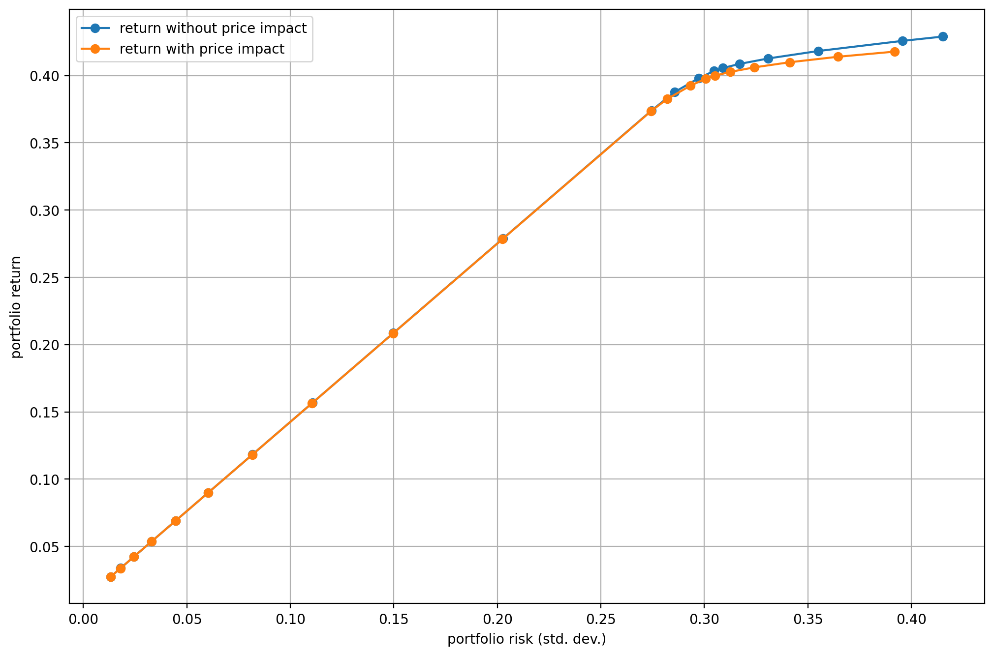
Fig. 6.1 The efficient frontier with risk-free security included, and market impact cost taken into account.

6.6.2 Transaction cost models

In this example we show a problem that models fixed and variable transaction costs and the buy-in threshold. Note that we do not model the market impact here.

We will assume now that $\mathbf{x}$ can take negative values too (short-selling is allowed), up to the limit of $30\mathrm{\%}$ portfolio size. This way we can see how to apply different costs to buy and sell trades. We also assume that ${\mathbf{x}}_0=\mathbf{0}$, so $\tilde{\mathbf{x}}=\mathbf{x}$.

The following code defines variables used as the positive and negative part variables of $\mathbf{x}$ and the binary variables ${\mathbf{y}}^{+},{\mathbf{y}}^{-}$ indicating whether there is buying or selling in a security:

# Real variables
xp = M.variable("xp", N, Domain.greaterThan(0.0))
xm = M.variable("xm", N, Domain.greaterThan(0.0))

# Binary variables
yp = M.variable("yp", N, Domain.binary())
ym = M.variable("ym", N, Domain.binary())

Next we add two constraints. The first links xp and xm to x, so that they represent the positive and negative parts. The second ensures that for each coordinate of yp and ym only one of the values can be $1$.

# Constraint assigning xp and xm to the positive and negative part of x.
M.constraint('pos-neg-part', x == xp - xm)

# Exclusive buy-sell constraint
M.constraint('exclusion', yp + ym <= 1.0)

We update the budget constraint with the variable and fixed transaction cost terms. The fixed cost of buy and sell trades are held by the variables fp and fm. These are typically given in dollars, and have to be divided by the total portfolio value. The variable cost coefficients are vp and vm. If these are given as percentages, then we do not have to modify them.

# Budget constraint with transaction cost terms
fixcost_terms = yp.T @ fp + ym.T @ fm
varcost_terms = xp.T @ vp + xm.T @ vm
budget_terms = Expr.sum(x) + varcost_terms + fixcost_terms
M.constraint('budget', budget_terms == 1.0)

Next, the 130/30 leverage constraint is added. Note that the transaction cost terms from the budget constraint should also appear here, otherwise the two constraints combined would allow a little more leverage than intended. (The sum of $\mathbf{x}$ would not reach $1$ because of the cost terms, leaving more space in the leverage constraint for negative positions.)

# Auxiliary variable for 130/30 leverage constraint
z = M.variable("z", N, Domain.unbounded())

# 130/30 leverage constraint
M.constraint('leverage-gt', z >= x)
M.constraint('leverage-ls', z >= -x)
M.constraint('leverage-sum',
             Expr.sum(z) + varcost_terms + fixcost_terms == 1.6)

Finally, to be able to differentiate between zero allocation (not incurring fixed cost) and nonzero allocation (incurring fixed cost), and to implement buy-in threshold, we need bound constraint involving the binary variables:

# Bound constraints
M.constraint('ubound-p', xp <= up * yp)
M.constraint('ubound-m', xm <= um * ym)
M.constraint('lbound-p', xp >= lp * yp)
M.constraint('lbound-m', xm >= lm * ym)

The full updated model will then look like the following:

def EfficientFrontier(N, m, G, deltas, vp, vm, fp, fm, up, um,
                      lp, lm, pcoef):
    with Model("TransactionCost") as M:
        # Real variables
        # The variable x is the fraction of holdings in each security.
        x = M.variable("x", N, Domain.unbounded())
        xp = M.variable("xp", N, Domain.greaterThan(0.0))
        xm = M.variable("xm", N, Domain.greaterThan(0.0))

        # Binary variables
        yp = M.variable("yp", N, Domain.binary())
        ym = M.variable("ym", N, Domain.binary())

        # Constraint assigning xp and xm to the pos. and neg. part of x.
        M.constraint('pos-neg-part', x == xp - xm)

        # s models the portfolio variance term in the objective.
        s = M.variable("s", 1, Domain.unbounded())

        # Auxiliary variable for 130/30 leverage constraint
        z = M.variable("z", N, Domain.unbounded())

        # Bound constraints
        M.constraint('ubound-p', xp <= up * yp)
        M.constraint('ubound-m', xm <= um * ym)
        M.constraint('lbound-p', xp >= lp * yp)
        M.constraint('lbound-m', xm >= lm * ym)

        # Exclusive buy-sell constraint
        M.constraint('exclusion', yp + ym <= 1.0)

        # Budget constraint with transaction cost terms
        fixcost_terms = yp.T @ fp + ym.T @ fm
        varcost_terms = xp.T @ vp + xm.T @ vm
        budget_terms = Expr.sum(x) + varcost_terms + fixcost_terms
        M.constraint('budget', budget_terms == 1.0)

        # 130/30 leverage constraint
        M.constraint('leverage-gt', z >= x)
        M.constraint('leverage-ls', z >= -x)
        M.constraint('leverage-sum',
                     Expr.sum(z) + varcost_terms + fixcost_terms == 1.6)

        # Objective (quadratic utility version)
        delta = M.parameter()
        penalty = pcoef * Expr.sum(xp + xm)
        M.objective('obj', ObjectiveSense.Maximize,
                           x.T @ m - penalty - delta * s)

        # Conic constraint for the portfolio variance
        M.constraint('risk', Expr.vstack(s, 1, G.T @ x),
                             Domain.inRotatedQCone())

        columns = ["delta", "obj", "return", "risk", "x_sum", "tcost"] + \
                  df_prices.columns.tolist()
        df_result = pd.DataFrame(columns=columns)
        for idx, d in enumerate(deltas):
            # Update parameter
            delta.setValue(d)

            # Solve optimization
            M.solve()

            # Save results
            portfolio_return = m @ x.level()
            portfolio_risk = np.sqrt(2 * s.level()[0])
            tcost = np.dot(vp, xp.level()) + np.dot(vm, xm.level()) + \
                    np.dot(fp, yp.level()) + np.dot(fm, ym.level())
            row = pd.Series([d, M.primalObjValue(), portfolio_return,
                             portfolio_risk, sum(x.level()), tcost] + \
                            list(x.level()), index=columns)
            df_result = df_result.append(row, ignore_index=True)

        return df_result

Here we also used a penalty term in the objective to prevent excess growth of the positive part and negative part variables. The coefficient of the penalty has to be calibrated so that we do not overpenalize.

We also have to mention that because of the binary variables, we can only solve this as a mixed integer optimization (MIO) problem. The solution of such a problem might not be as efficient as the solution of a problem with only continuous variables. See Sec. 13.2 (Mixed-integer models) for details regarding MIO problems.

We compute the efficient frontier with and without transaction costs. The following code produces the results:

deltas = np.logspace(start=-0.5, stop=2, num=20)[::-1]
ax = plt.gca()
for a in [0, 1]:
    pcoef = a * 0.03
    fp = a * 0.005 * np.ones(N) # Depends on portfolio value
    fm = a * 0.01 * np.ones(N) # Depends on portfolio value
    vp = a * 0.01 * np.ones(N)
    vm = a * 0.02 * np.ones(N)
    up = 2.0
    um = 2.0
    lp = a * 0.05
    lm = a * 0.05

    df_result = EfficientFrontier(N, m, G, deltas, vp, vm, fp, fm, up, um,
                                  lp, lm, pcoef)
    df_result.plot(ax=ax, x="risk", y="return", style="-o",
                   xlabel="portfolio risk (std. dev.)",
                   ylabel="portfolio return", grid=True)
ax.legend(["return without transaction cost",
          "return with transaction cost"])

On Fig. 6.2 we can see the return reducing effect of transaction costs. The overall return is higher because of the leverage.

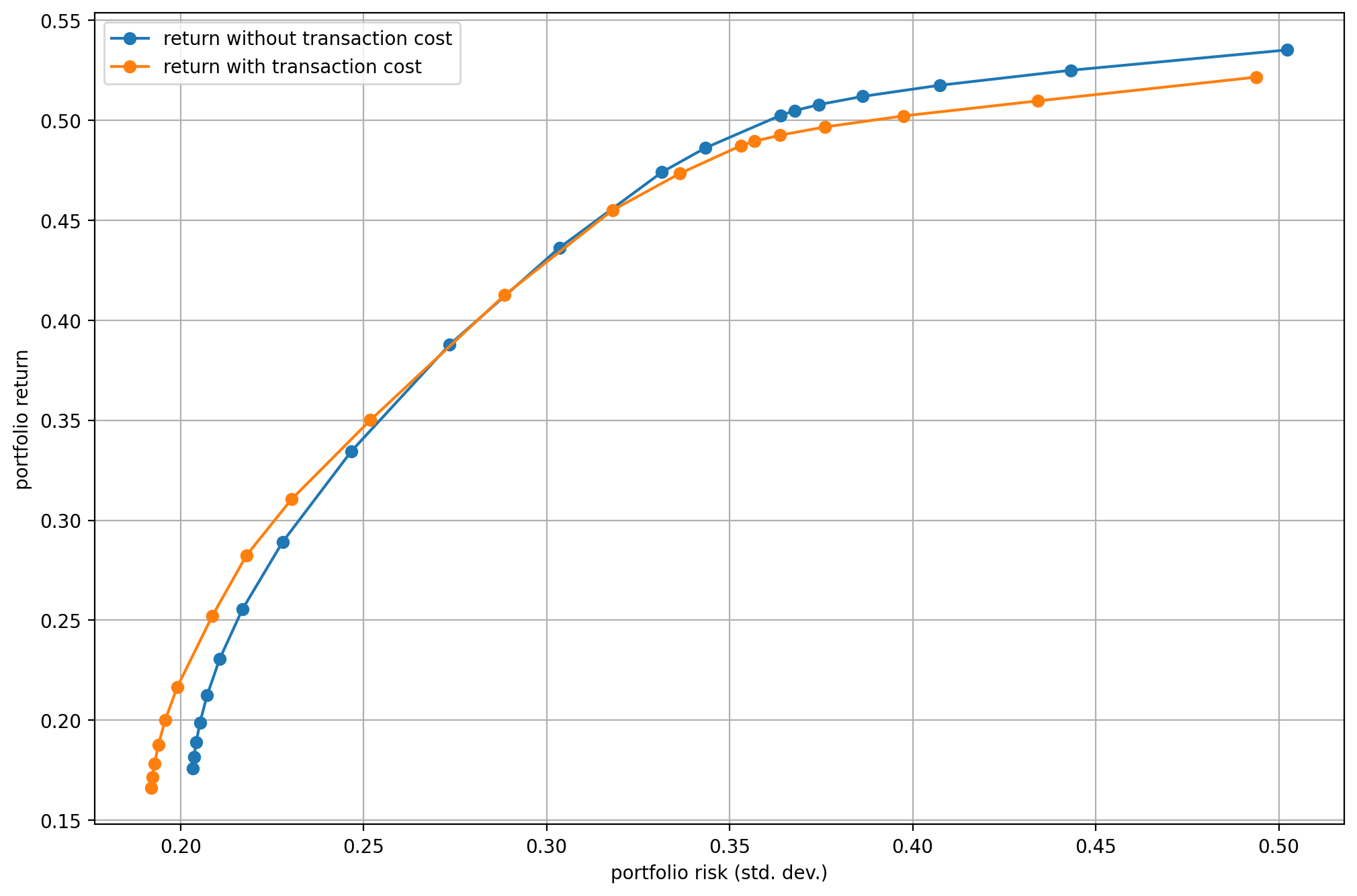
Fig. 6.2 The efficient frontier with transaction costs taken into account.