9 Risk budgeting

Traditional MVO only considers the risk of the portfolio and ignores how the risk is distributed among individual securities. This might result in risk being concentrated into only a few securities, when these gain too much weight in the portfolio.

Risk budgeting techniques were developed to give portfolio managers more control over the amount of risk each security contributes to the total portfolio risk. They allocate the risk instead of the capital, thus diversify risk more directly. Risk budgeting also makes the resulting portfolio less sensitive to estimation errors, because it excludes the use of expected return estimates [CK20, Pal20].

9.1 Risk contribution

If the risk measure is a homogeneous function of degree one, then we can use Euler decomposition write the total portfolio risk \(\mathcal{R}_\mathbf{x}\) as the sum of risk contributions \(\mathrm{rc}_{\mathbf{x},i}\) of each security:

(9.1)\[\mathcal{R}_\mathbf{x} = \sum_{i=1}^N \mathrm{rc}_{\mathbf{x},i} = \sum_{i=1}^N x_i \mathrm{mrc}_{\mathbf{x},i} = \sum_{i=1}^N x_i \frac{\partial\mathcal{R}_\mathbf{x}}{\partial x_i} = \mathbf{x}^\mathsf{T}\nabla\mathcal{R}_\mathbf{x}\]

where \(\mathrm{mrc}_{\mathbf{x},i} = \frac{\partial\mathcal{R}_\mathbf{x}}{\partial x_i}\) is called marginal risk contribution, because it measures the sensitivity of the portfolio standard deviation to changes in \(x_i\).

9.2 Risk budgeting portfolio

With the above definitions, the risk budgeting portfolio aims to allocate the risk contributions according to a predetermined risk profile \(\mathbf{b}\). In other words, it aims to find the portfolio \(\mathbf{x}\) that solves the system

(9.2)\[\mathbf{x}\circ\nabla\mathcal{R}_\mathbf{x} = \mathbf{b}\circ\mathcal{R}_\mathbf{x} = \mathbf{b}\circ\mathbf{x}^\mathsf{T}\nabla\mathcal{R}_\mathbf{x}\]

where \(\mathbf{1}^\mathsf{T}\mathbf{b} = 1\) and \(\mathbf{b} \geq \mathbf{0}\). A special case of this is the risk parity portfolio, for which \(b_i = \frac{1}{N}\).

Using that \(\nabla\mathcal{R}_\mathbf{cx} = \nabla\mathcal{R}_\mathbf{x}\) for homogeneous \(\mathcal{R}_\mathbf{x}\) of degree one and \(c\in\R\), we can see that if \(\mathbf{x}_\mathrm{rb}\) is a risk budgeting portfolio, then so is \(c\mathbf{x}_\mathrm{rb}\). In some solution approaches it is useful to define a risk-normalized variable \(\mathbf{y} = \mathbf{x}/\mathcal{R}_\mathbf{x}\), and get

(9.3)\[\mathbf{y}\circ\nabla\mathcal{R}_\mathbf{y} = \mathbf{b}\]

Working with this form is typically easier. After solving these equations, we can recover the portfolio \(\mathbf{x}\) by normalizing again.

9.3 Risk budgeting with variance

If we use portfolio variance as risk measure, i. e., set \(\mathcal{R}_\mathbf{x} = \mathbf{x}^\mathsf{T}\ECov\mathbf{x}\), then (9.2) will become

(9.4)\[\mathbf{x}\circ\ECov\mathbf{x} = \mathbf{b}\circ\mathbf{x}^\mathsf{T}\ECov\mathbf{x},\]

and (9.3) will become

(9.5)\[\mathbf{y}\circ\ECov\mathbf{y} = \mathbf{b}\]

Solving this system is inherently a non-convex problem because it has quadratic equality constraints. However, we can still formulate convex optimization problems to find the solution.

In general, however, we have to be aware that the conditions defining the risk budgeting portfolio are very restrictive. Therefore we have very limited possibility to further constrain a risk budgeting problem, without making the risk budgeting portfolio infeasible.

9.3.1 Convex formulation using quadratic cone

Suppose we allocate the risk budget \(b_m\) for each security \(i\) in a group of securities \(\mathcal{G}_m\), and we have \(M\) such groups. As special cases, we have \(M = N\) when each security has a unique risk budget, thus each \(\mathcal{G}_m\) contains only one security. In contrast, we have \(M = 1\) when all risk budgets \(b_i = 1/N\) are the same, leading to the risk parity portfolio.

Let us now focus on group \(\mathcal{G}_m\). We can define new variables \(\gamma_{\mathrm{u},m}\) and \(\gamma_{\mathrm{l},m}\) to bound the risk contributions in this group from above and from below. First we express the risk contributions as the fraction of the total risk \(b_m\mathbf{x}^\mathsf{T}\ECov\mathbf{x}\). We can bound this from above to get the constraint

\[b_m\mathbf{x}^\mathsf{T}\ECov\mathbf{x} \leq \gamma_{\mathrm{u},m}^2,\]

and model it using the quadratic cone.

Next, we bound the risk contributions from below as

\[x_i(\ECov \mathbf{x})_i \geq \gamma_{\mathrm{l},m}^2.\]

Assuming \(x_i \geq 0\) and \((\ECov \mathbf{x})_i \geq 0\), we can model this using the power cone as \((x_i, (\ECov \mathbf{x})_i, \gamma_{\mathrm{l},m}) \in \POW_3^{1/2,1/2}\), or equivalently using the rotated quadratic cone as \((x_i/\sqrt{2}, (\ECov \mathbf{x})_i/\sqrt{2}, \gamma_{\mathrm{l},m}) \in \Q_\mathrm{r}^3\).

Finally, minimizing the difference between the upper and lower bounds, we get the risk budgeting portfolio as the optimal solution. The full optimization problem will look like

(9.6)\[\begin{split}\begin{array}{lrcl} \mbox{minimize} & \sum_{m=1}^M \gamma_{\mathrm{u},m} - \gamma_{\mathrm{l},m} & & \\ \mbox{subject to} & \mathbf{1}^\mathsf{T}\mathbf{x} & = & 1,\\ & (\gamma_{\mathrm{u},m}/\sqrt{b_m}, \mathbf{G}^\mathsf{T}\mathbf{x}) & \in & \Q^{k+1},\quad m=1,\dots,M, \\ & (x_i, (\ECov\mathbf{x})_i, \gamma_{\mathrm{l},m}) & \in & \POW_3^{1/2,1/2},\quad i \in \mathcal{G}_m,\ m=1,\dots,M, \\ & \mathbf{x}, \ECov\mathbf{x} & \geq & \mathbf{0},\\ & \gamma_{\mathrm{u},m} & \geq & \gamma_{\mathrm{l},m},\quad m=1,\dots,M, \end{array}\end{split}\]

where \(\ECov = \mathbf{G}\mathbf{G}^\mathsf{T}\) for \(\mathbf{G} \in \R^{N\times k}\).

Note that we have to be careful adding further constraints to problem (9.6), because these might make the risk budgeting portfolio infeasible.

9.3.2 Convex formulation using exponential cone

There also exists a different convex formulation of the risk budgeting problem, that works not only in the positive orthant, but in any (prespecified) orthant of the portfolio space. This allows us to work with long-short portfolios as well.

Observe that the risk budgeting equations (9.4) are the first-order optimality conditions of the optimization problem

(9.7)\[\begin{split}\begin{array}{lrcl} \mbox{minimize} & \frac{1}{2}\mathbf{x}^\mathsf{T}\ECov\mathbf{x} - c\mathbf{b}^\mathsf{T}\log\left(\mathbf{z}\circ\mathbf{x}\right) & & \\ \mbox{subject to} & \mathbf{z}\circ\mathbf{x} & \geq & \mathbf{0}. \end{array}\end{split}\]

We can use the parameter \(c\) to scale the sum of vector \(\mathbf{b}\), leading to different magnitude of the optimal solution. Thus we can directly find a solution that satisfies for example \(\sum_i x_i = 1\) or in the long-short case \(\sum_i |x_i| = 1\).

Problem (9.7) can be modeled using the exponential cone in the following way:

(9.8)\[\begin{split}\begin{array}{lrcl} \mbox{minimize} & s - c\mathbf{b}^\mathsf{T}\mathbf{t} & & \\ \mbox{subject to} & (s, 1, \mathbf{G}^\mathsf{T}\mathbf{x}) & \in & \Q_\mathrm{r}^{k+2}, \\ & (z_ix_i, 1, t_i) & \in & \EXP,\quad i=1,\dots,N, \\ & \mathbf{z}\circ\mathbf{x} & \geq & \mathbf{0}, \end{array}\end{split}\]

where \(\ECov = \mathbf{G}\mathbf{G}^\mathsf{T}\) for \(\mathbf{G} \in \R^{N\times k}\).

While this convex approach works with any sign configuration \(\mathbf{z}\in \{+1, -1\}^N\) of \(\mathbf{x}\), we have to specify \(\mathbf{z}\) as parameter, meaning we can still only compute the optimal solution for a given orthant. The reason is that by design, there are solutions to (9.4) in each orthant. There are \(2^{N}\) (normalized) solutions, one for each possible \(\mathbf{z}\circ\mathbf{x} > 0\) [CK20], i. e., one in each orthant. [1] So there is a local optimal solution in each orthant, meaning that the problem is non-convex on the full space.

Also note that in this formulation we cannot add further constraints, because these could alter the optimality conditions (9.4), making the solution invalid as a risk budgeting portfolio.

9.3.3 Mixed integer formulation

In each orthant, the solution to (9.7) can have a different total risk. Therefore we can try to find a risk budgeting portfolio that has low total risk. In order to do this, we can extend problem (9.7) to be mixed integer. This will allow us to optimize over the full space, including all long-short portfolios, without needing to prespecify the signs. After defining separate variables based on Sec. 13.2.1.4 (Positive and negative part) for the long and the short part of the portfolio, we get:

(9.9)\[\begin{split}\begin{array}{lrcl} \mbox{minimize} & \frac{1}{2}\mathbf{x}^\mathsf{T}\ECov\mathbf{x} - c\mathbf{b}^\mathsf{T}\log\left(\mathbf{x}^++\mathbf{x}^-\right) & & \\ \mbox{subject to} & \mathbf{x}^+, \mathbf{x}^- & \geq & 0, \\ & \mathbf{x} & = & \mathbf{x}^+ - \mathbf{x}^-,\\ & \mathbf{x}^+ & \leq & M\mathbf{z}^+,\\ & \mathbf{x}^- & \leq & M\mathbf{z}^-,\\ & \mathbf{z}^+ + \mathbf{z}^- & \leq & \mathbf{1},\\ & \mathbf{z}^+, \mathbf{z}^- & \in & \{0, 1\}^N. \end{array}\end{split}\]

What makes sure that problem (9.9) will find a low risk solution? The first term of the objective function is the sum of risk budgets, thus in any optimal solution, we must have \(\mathbf{x}^\mathsf{T}\ECov\mathbf{x} = \sqrt{c}\), because the risk budgeting conditions are satisfied. It follows that the second term will decide the optimal objective value. This logarithmic term will become the lowest if the monomial \(\mathbf{|x|}^{c\mathbf{b}} = \left(\|\mathbf{x}\|_1 |\hat{\mathbf{x}}|^\mathbf{b}\right)^c\) is largest, where \(\hat{\mathbf{x}}\) denotes a unit vector. Depending on \(\mathbf{b}\), this implies an optimal \(\mathbf{x}\) with large 1-norm. It follows that after normalization, this \(\mathbf{x}\) will yield a low value for the total risk \(\mathbf{x}^\mathsf{T}\ECov\mathbf{x}\). Note however, that it is not guaranteed to get the lowest risk, because \(|\hat{\mathbf{x}}|^\mathbf{b}\) can also vary.

A further tradeoff with the mixed integer approach is that we have no performance guarantee, finding the optimal solution can take a lot of time. Most likely we will have to settle with suboptimal portfolios in terms of risk.

9.4 Example

In this example we show how can we find a risk parity portfolio by solving a convex optimization problem in MOSEK Fusion.

The input data is again obtained the same way as detailed in Sec. 3.4.2 (Data collection). Here we assume that the covariance matrix estimate \(\ECov\) of yearly returns is available.

The optimization problem we solve here is (9.8), which we repeat here:

(9.10)\[\begin{split}\begin{array}{lrcl} \mbox{minimize} & s - c\mathbf{b}^\mathsf{T}\mathbf{t} & & \\ \mbox{subject to} & (s, 1, \mathbf{G}^\mathsf{T}\mathbf{x}) & \in & \Q_\mathrm{r}^{k+2}, \\ & (z_ix_i, 1, t_i) & \in & \EXP,\quad i=1,\dots,N, \\ & \mathbf{z}\circ\mathbf{x} & \geq & \mathbf{0}, \end{array}\end{split}\]

We search for a solution in the positive orthant, so we set \(\mathbf{z} = \mathbf{1}\). We choose the risk budget vector to be \(\mathbf{b}=1/N\), so that all securities contribute the same amount of risk.

The Fusion model of (9.10):

def RiskBudgeting(N, G, b, z, a):

 with Model('Risk budgeting') as M:
     # Settings
     M.setLogHandler(sys.stdout)

     # Portfolio weights
     x = M.variable("x", N, Domain.unbounded())

     # Orthant specifier constraint
     M.constraint("orthant", Expr.mulElm(z, x), Domain.greaterThan(0.0))

     # Auxiliary variables
     t = M.variable("t", N, Domain.unbounded())
     s = M.variable("s", 1, Domain.unbounded())

     # Objective function: 1/2 * x'Sx - a * b'log(z*x) becomes s - a * b't
     M.objective(ObjectiveSense.Minimize,
         Expr.sub(s, Expr.mul(a, Expr.dot(b, t))))

     # Bound on risk term
     M.constraint(Expr.vstack(s, 1, Expr.mul(G.T, x)),
         Domain.inRotatedQCone())

     # Bound on log term t <= log(z*x) becomes (z*x, 1, t) in K_exp
     M.constraint(Expr.hstack(Expr.mulElm(z, x),
                  Expr.constTerm(N, 1.0),
                  t),
         Domain.inPExpCone())

     # Create DataFrame to store the results.
     columns = ["obj", "risk", "xsum", "bsum"] + df_prices.columns.tolist()
     df_result = pd.DataFrame(columns=columns)

     # Solve optimization
     M.solve()

     # Save results
     xv = x.level()

     # Check solution quality
     risk_budgets = xv * np.dot(G @ G.T, xv)

     # Renormalize to gross exposure = 1
     xv = xv / np.abs(xv).sum()

     # Compute portfolio metrics
     Gx = np.dot(G.T, xv)
     portfolio_risk = np.sqrt(np.dot(Gx, Gx))

     row = pd.Series([M.primalObjValue(), portfolio_risk, np.sum(z * xv),
         np.sum(risk_budgets)] + list(xv), index=columns)
     df_result = df_result.append(row, ignore_index=True)
     row = pd.Series([None] * 4 + list(risk_budgets), index=columns)
     df_result = df_result.append(row, ignore_index=True)

     return df_result

The following code defines the parameters, including the matrix \(\mathbf{G}\) such that \(\ECov=\mathbf{G}\mathbf{G}^T\).

# Number of securities
N = 8
# Risk budget
b = np.ones(N) / N
# Orthant selector
z = np.ones(N)
# Global setting for sum of b
c = 1
# Cholesky factor of the covariance matrix S
G = np.linalg.cholesky(S)

Finally, we produce the optimization results:

df_result = RiskBudgeting(N, G, b, z, c)

On Fig. 9.1 we can see the portfolio composition, and on Fig. 9.2 the risk contributions of each security.

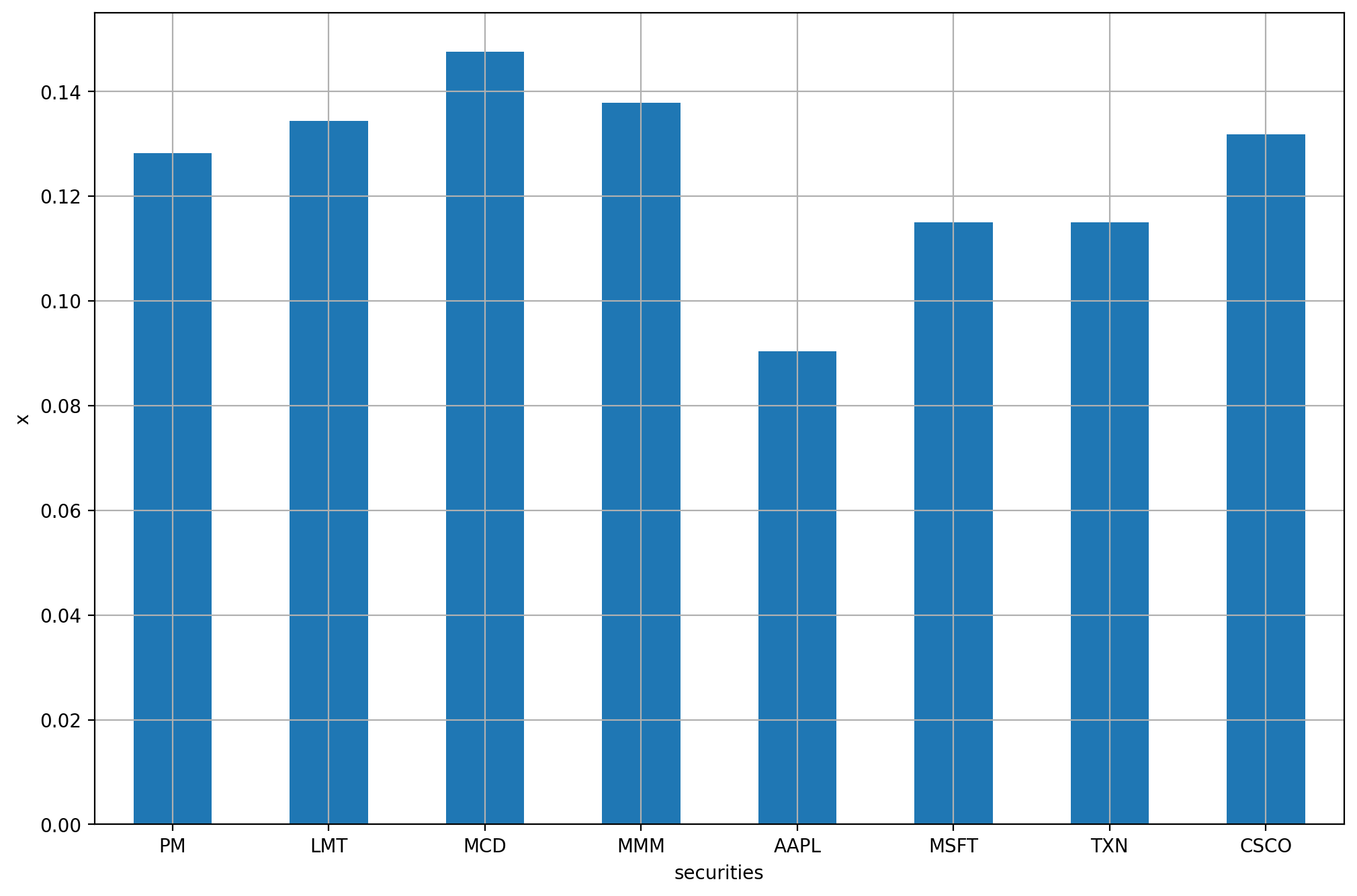
Fig. 9.1 The risk budgeting portfolio.

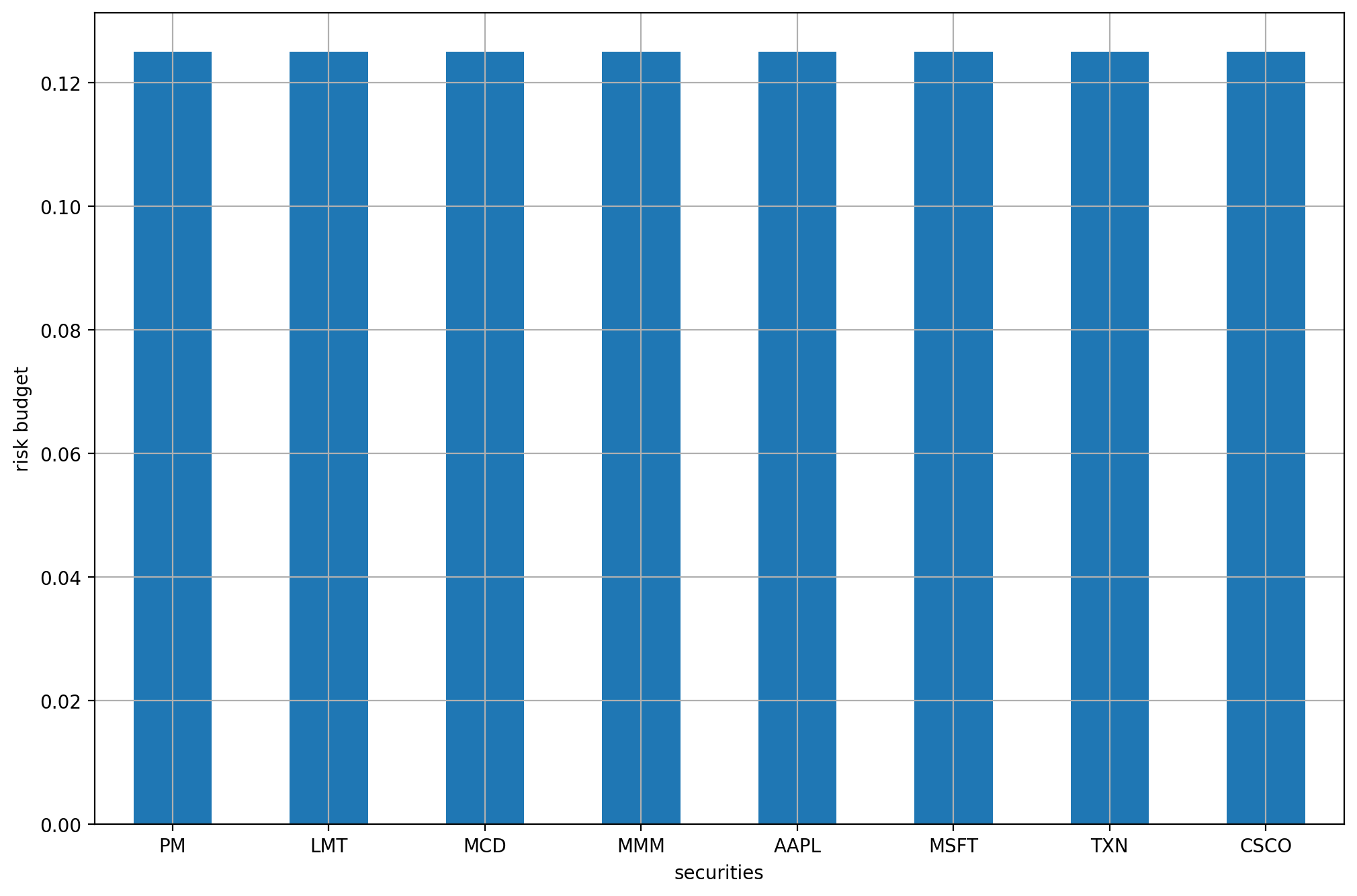
Fig. 9.2 The risk contributions of each security.

Footnotes

[1]

Of course the solutions in opposite orthants differ only by global sign, so these can be considered the same solution.