8 Other risk measures

In the definitions (2.1)-(2.4) of the classical MVO problem the variance (or standard deviation) of portfolio return is used as the measure of risk, making computation easy and convenient. If we assume that the portfolio return is normally distributed, then the variance is in fact the optimal risk measure, because then MVO can take into account all information about return. Moreover, if $T$ is large compared to $N$, the sample mean and covariance matrix are maximum likelihood estimates (MLE), implying that the optimal portfolio resulting from estimated inputs will also be a MLE of the true optimal portfolio [Lau01].

Empirical observations suggest however, that the distribution of linear return is often skewed, and even if it is elliptically symmetric, it can have fat tails and can exhibit tail dependence [1]. As the distribution moves away from normality, the performance of a variance based portfolio estimator can quickly degrade.

No perfect risk measure exists, though. Depending on the distribution of return, different measures can be more appropriate in different situations, capturing different characteristics of risk. Return of diversified equity portfolios are often approximately symmetric over periods of institutional interest. Options, swaps, hedge funds, and private equity have return distributions that are unlikely to be symmetric. Also less symmetric are distributions of fixed-income and real estate index returns, and diversified equity portfolios over long time horizons [MM08].

The measures presented here are expectations, meaning that optimizing them would lead to stochastic optimization problems in general. As a simplification, we consider only their sample average approximation by assuming that a set of linear return scenarios are given.

8.1 Deviation measures

This class of measures quantify the variability around the mean of the return distribution, similar to variance. If we associate investment risk with the uncertainty of return, then such measures could be ideal.

Let $X,Y$ be random variables of investment returns, and let $D$ be a mapping. The general properties that deviation measures should satisfy are [RUZ06]:

1. Positivity: $D(X)\ge 0$ with $D(X)=0$ only if $X=c\in \mathbb{R}$,

2. Translation invariance: $D(X+c)=D(X),c\in \mathbb{R}$,

3. Subadditivity: $D(X+Y)\le D(X)+D(Y)$,

4. Positive homogeneity: $D(cX)=cD(X),c\ge 0$

Note that positive homegeneity and subadditivity imply the convexity of $D$.

8.1.1 Robust statistics

A group of deviation measures are robust statistics. Maximum likelihood estimators are highly sensitive to deviations from the assumed distribution. Thus if the return is not normally distributed, robust portfolio estimators can be an alternative. These are less efficient than MLE for normal distribution, but their performance degrades less quickly under departures from normality. One suitable class of estimators to express portfolio risk are M-estimators [VD09]:

$$D_{\delta }(R_{\mathbf{x}})=\underset{q}{min}\mathbb{E}[\delta (R_{\mathbf{x}}-q)],$$

where $\delta$ is a convex loss function with unique minimum at zero. It has the sample average approximation $\underset{q}{min}\frac{1}{T}\sum _{k=1}^T\delta ({\mathbf{x}}^{\mathsf{T}}{\mathbf{r}}_k-q)$.

8.1.1.1 Variance

Choosing ${\delta }_{\mathrm{var}}(y)=\frac{1}{2}{y}^2$ we get $D_{{\delta }_{\mathrm{var}}}$, a different expression for the portfolio variance. The optimal $q$ in this case is the portfolio mean return ${\mu }_{\mathbf{x}}$. This gives us a way to perform standard mean–variance optimization directly using scenario data, without the need for a sample covariance matrix:

(8.1)$$\begin{array}{r}\begin{array}{lrcl}\text{minimize}& \frac{1}{2T}\sum _{k=1}^T({\mathbf{x}}^{\mathsf{T}}{\mathbf{r}}_k-q{)}^2& & \\ \text{subject to}& \mathbf{x}& \in & \mathcal{F}.\end{array}\end{array}$$

By defining new variables $t_k^{+}=\max ({\mathbf{x}}^{\mathsf{T}}{\mathbf{r}}_k-q,0)$ and $t_k^{-}=\max (-{\mathbf{x}}^{\mathsf{T}}{\mathbf{r}}_k+q,0)$, then using Sec. 13.1.1.1 (Maximum function) we arrive at a QO model:

(8.2)$$\begin{array}{r}\begin{array}{lrcl}\text{minimize}& \frac{1}{2T}\Vert {\mathbf{t}}^{+}{\Vert }^2+\frac{1}{2T}\Vert {\mathbf{t}}^{-}{\Vert }^2& & \\ & {\mathbf{x}}^{\mathsf{T}}\mathbf{R}-q& =& {\mathbf{t}}^{+}-{\mathbf{t}}^{-},\\ & {\mathbf{t}}^{+},{\mathbf{t}}^{-}& \ge & 0,\\ \text{subject to}& \mathbf{x}& \in & \mathcal{F},\end{array}\end{array}$$

where $\mathbf{R}=[{\mathbf{r}}_1,\dots ,{\mathbf{r}}_T]$ is the scenario matrix, where each column is a scenario. The norms can be further modeled by the rotated quadratic cone; see in Sec. 13.1.1.9 (Squared Euclidean norm). While this formulation does not need covariance estimation, it can still suffer from computational inefficiency because the number of variables and the number of constraints depend on the sample size $T$.

8.1.1.2 $\alpha$-shortfall

Choosing ${\delta }_{\mathrm{sf},\alpha }(y)=\alpha y-\min (y,0)$ or equivalently ${\delta }_{\mathrm{sf},\alpha }(y)=\alpha \max (y,0)+(1-\alpha )\max (-y,0)$ for $\alpha \in (0,1)$ will give the $\alpha$-shortfall $D_{{\delta }_{\mathrm{sf},\alpha }}$ studied in [Lau01]. The optimal $q$ will be the $\alpha$-quantile of the portfolio return. $\alpha$-shortfall is a deviation measure with favorable robustness properties when the portfolio return has an asymmetric distribution, fat tailed symmetric distribution, or exhibits multivariate tail-dependence. The $\alpha$ parameter adjusts the level of asymmetry in the $\delta$ function, allowing us to penalize upside and downside returns differently.

Portfolio optimization using sample $\alpha$-shortfall can be formulated as

(8.3)$$\begin{array}{r}\begin{array}{lrcl}\text{minimize}& \frac{\alpha }{T}\sum _{k=1}^T({\mathbf{x}}^{\mathsf{T}}{\mathbf{r}}_k-q)-\frac{1}{T}\sum _{k=1}^T\min ({\mathbf{x}}^{\mathsf{T}}{\mathbf{r}}_k-q,0)& & \\ \text{subject to}& \mathbf{x}& \in & \mathcal{F}\end{array}\end{array}$$

By defining new variables $t_k^{-}=\max (-{\mathbf{x}}^{\mathsf{T}}{\mathbf{r}}_k+q,0)$, and model accoring to Sec. 13.1.1.1 (Maximum function) we arrive at an LO model:

(8.4)$$\begin{array}{r}\begin{array}{lr}\text{minimize}& \alpha ({\mathbf{x}}^{\mathsf{T}}\mathit{\mu }-q)+\frac{1}{T}\sum _{k=1}^T{t}_k^{-}\\ & {\mathbf{t}}^{-}& \ge & -{\mathbf{x}}^{\mathsf{T}}{\mathbf{r}}_k+q,\\ & {\mathbf{t}}^{-}& \ge & 0,\\ \text{subject to}& \mathbf{x}& \in & \mathcal{F}.\end{array}\end{array}$$

A drawback of this model is that the number of constraints depends on the sample size $T$, resulting in computational inefficiency for large number of samples.

For elliptically symmetric return distributions the $\alpha$-shortfall is equivalent to the variance in the sense that the corresponding sample portfolio estimators will be estimating the same portfolio. In fact for normal distribution, the $\alpha$-shortfall is proportional to the portfolio variance: $D_{{\delta }_{\mathrm{sf},\alpha }}=\frac{\varphi (q_{\alpha })}{\alpha }\sqrt{D_{{\delta }_{\mathrm{var}}}}$, where $\varphi (q_{\alpha })$ is the value of the standard normal density function at its $\alpha$-quantile.

However when return is symmetric but not normally distributed, the sample portfolio estimators for $\alpha$-shortfall can have less estimation error than sample portfolio estimators for variance.

8.1.1.3 MAD

A special case of $\alpha$-shortfall is for $\alpha =0.5$. The function ${\delta }_{\mathrm{MAD}}(y)=\frac{1}{2}|y|$ gives us $D_{{\delta }_{\mathrm{MAD}}}$, which is called the mean absolute deviation (MAD) measure or the $L_1$-risk. For this case the optimal $q$ will be the median of the portfolio return, and the sample MAD portfolio optimization problem can be formulated as

(8.5)$$\begin{array}{r}\begin{array}{lrcl}\text{minimize}& \frac{1}{2T}\sum _{k=1}^T|{\mathbf{x}}^{\mathsf{T}}{\mathbf{r}}_k-q|& & \\ \text{subject to}& \mathbf{x}& \in & \mathcal{F}.\end{array}\end{array}$$

After modeling the absolute value based on Sec. 13.1.1.3 (Absolute value) we arrive at the following LO:

(8.6)$$\begin{array}{r}\begin{array}{lrcl}\text{minimize}& \frac{1}{2T}\sum _{k=1}^T{t}_k& & \\ \text{subject to}& {\mathbf{x}}^{\mathsf{T}}\mathbf{R}-q& \ge & -\mathbf{t},\\ & {\mathbf{x}}^{\mathsf{T}}\mathbf{R}-q& \le & \mathbf{t},\\ & \mathbf{x}& \in & \mathcal{F},\end{array}\end{array}$$

where $\mathbf{R}$ is the return data matrix with one observation ${\mathbf{r}}_k,k=1,\dots ,T$ in each column. Note that the number of constraints in this LO problem again depends on the sample size $T$.

For normally distributed returns, the MAD is proportional to the variance: $D_{{\delta }_{MAD}}=\sqrt{\frac{2}{\pi }}\sqrt{D_{{\delta }_{\mathrm{var}}}}$.

The $L_1$-risk can also be applied without minimizing over $q$. We can just let $q$ to be the sample portfolio mean instead, i. e., $q={\mathbf{x}}^{\mathsf{T}}\mathit{\mu }$ [KY91].

8.1.1.4 Risk measure from the Huber function

Another robust portfolio estimator can be obtained for the case of symmetric return distributions using the Huber function

$$\begin{array}{r}{\delta }_{\mathrm{H}}(y)=\{\begin{array}{ll}{y}^2,& |y|\le c\\ 2c|y|-c^2,& |y|>c\end{array},\end{array}$$

yielding the risk measure $D_{{\delta }_{\mathrm{H}}}$. A different form of the Huber function is ${\delta }_{\mathrm{H}}(y)={\min }_u{u}^2+2c|y-u|$, which leads to a QO formulation:

(8.7)$$\begin{array}{r}\begin{array}{lrcl}\text{minimize}& \frac{1}{T}\sum _{k=1}^T{u}_k^2+\frac{1}{T}\sum _{k=1}^{T}2c|{\mathbf{x}}^{\mathsf{T}}{\mathbf{r}}_k-q-u_k|& & \\ \text{subject to}& \mathbf{x}& \in & \mathcal{F}.\end{array}\end{array}$$

Modeling the absolute value based on Sec. 13.1.1.3 (Absolute value) we get

(8.8)$$\begin{array}{r}\begin{array}{lrcl}\text{minimize}& \frac{1}{T}\sum _{k=1}^T{u}_k^2+\frac{1}{T}\sum _{k=1}^{T}2c{t}_k& & \\ \text{subject to}& {\mathbf{x}}^{\mathsf{T}}\mathbf{R}-q-\mathbf{u}& \ge & -\mathbf{t},\\ & {\mathbf{x}}^{\mathsf{T}}\mathbf{R}-q-\mathbf{u}& \le & \mathbf{t},\\ & \mathbf{x}& \in & \mathcal{F}.\end{array}\end{array}$$

Note that the size of this problem depends on the number of samples $T$.

8.1.2 Downside deviation measures

In financial context many distributions are skewed. Investors might only be concerned with negative deviations (losses) relative to the expected portfolio return ${\mu }_{\mathbf{x}}$, or in general with falling short of some benchmark return $r_{\mathrm{bm}}$. In these cases downside deviation measures are more appropriate.

A class of downside deviation measures are lower partial moments of order $n$:

$${\mathrm{LPM}}_n(r_{\mathrm{bm}})=\mathbb{E}(\max (r_{\mathrm{bm}}-R_{\mathbf{x}},0{)}^n),$$

where $r_{\mathrm{bm}}$ is some given target return. The discrete version of this measure is $\sum _{k=1}^T{p}_k\max (r_{\mathrm{bm}}-{\mathbf{x}}^{\mathsf{T}}{\mathbf{r}}_k,0{)}^n,$ where ${\mathbf{r}}_k$ is a scenario of the portfolio return $R_{\mathbf{x}}$ occurring with probability $p_k$.

We have the following special cases:

• ${\mathrm{LPM}}_0$ is the probability of loss relative to the target return $r_{\mathrm{bm}}$. ${\mathrm{LPM}}_0$ is an incomplete measure of risk, because it does not provide any indication of how severe the shortfall can be, should it occur. Therefore it is best used as a constraint while optimizing for a different risk measure. This way ${\mathrm{LPM}}_0$ can still provide information about the risk tolerance of the investor.

• ${\mathrm{LPM}}_1$ is the expected loss, also called target shortfall.

• ${\mathrm{LPM}}_2$ is called target semi-variance.

While lower partial moments only consider outcomes below the target $r_{\mathrm{bm}}$, the optimization still uses the entire distribution of $R_{\mathbf{x}}$. The right tail of the distribution (representing the outcomes above the target) is captured in the mean ${\mu }_{\mathbf{x}}$ of the distribution.

The ${\mathrm{LPM}}_n$ optimization problem can be formulated as [Lau01]

(8.9)$$\begin{array}{r}\begin{array}{lrcl}\text{minimize}& \sum _{k=1}^T{p}_k\max (r_{\mathrm{bm}}-{\mathbf{x}}^{\mathsf{T}}{\mathbf{r}}_k,0{)}^n& & \\ \text{subject to}& \mathbf{x}& \in & \mathcal{F}.\end{array}\end{array}$$

If we define the new variables $t_k^{-}=\max (r_{\mathrm{bm}}-{\mathbf{x}}^{\mathsf{T}}{\mathbf{r}}_k,0)$, then for $n=1$ we arrive at an LO and for $n=2$ we arrive at a QO problem:

(8.10)$$\begin{array}{r}\begin{array}{lrcl}\text{minimize}& \sum _{k=1}^T{p}_k(t_k^{-}{)}^n& & \\ \text{subject to}& {\mathbf{t}}^{-}& \ge & r_{\mathrm{bm}}-{\mathbf{x}}^{\mathsf{T}}\mathbf{R},\\ & {\mathbf{t}}^{-}& \ge & 0,\\ & \mathbf{x}& \in & \mathcal{F},\end{array}\end{array}$$

where ${\mathbf{t}}^{-}$ is $T$ dimensional vector. Thus there will be $N+T$ variables, and the number of constraints will also depend on the sample size $T$.

Contrary to the variance, ${\mathrm{LPM}}_n$ measures are consistent with more general classes of investor utility functions, and assume less about the return distribution. Thus they better reflect investor preferences and are valid under a broader range of conditions [Har91].

However, LPMs are only useful for skewed distributions. If the return distribution is symmetric, ${\mathrm{LPM}}_1$ and ${\mathrm{LPM}}_2$ based portfolio estimates will be equivalent to MAD and variance based ones. In particular the MAD for a random variable with density $f(x)$ will be the same as ${\mathrm{LPM}}_1$ of a random variable with density $f(x)+f(-x)$. Also, the mean-LPM optimization model is very sensitive to the changes in the target value.

8.2 Tail risk measures

Tail risk measures try to capture the risk of extreme events. The measures described below are commonly defined for random variables treating loss as positive number, so to apply them on security returns $R$ we have to flip the sign and define loss as $L=-R$.

Let $X,Y$ be random variables of investment losses, and let $\tau$ be a mapping. The formal properties that a reasonable tail risk measure should satisfy are the following [FS02]:

1. Monotonicity: If $X\le Y$, then $\tau (X)\le \tau (Y)$,

2. Translation invariance: $\tau (X+m)=\tau (X)+m,m\in \mathbb{R}$,

3. Subadditivity: $\tau (X+Y)\le \tau (X)+\tau (Y)$,

4. Positive homogeneity: $\tau (cX)=c\tau (X),c\ge 0$

If $\tau$ satisfies these properties then it is called coherent risk measure. If we relax condition 3 and 4 to the property of convexity, then we get the more general class of convex risk measures. Not all risk measures used in practice satisfy these properties, violation of condition 1 and/or 2 is typical. However, in the context of portfolio selection these are less critical, the property of convexity is most important to achieve risk diversification [Lau01].

8.2.1 Value-at-Risk

Denote the $\alpha$-quantile of a random variable $L$ by $q_{\alpha }(L)=\inf \{x|\mathbb{P}(L\le x)\ge \alpha \}$. If $L$ is the loss over a given time horizon, then the value-at-risk (VaR) of $L$ with confidence level $\alpha$ (or risk level $1-\alpha$) is defined to be

$${\mathrm{VaR}}_{\alpha }(L)=q_{\alpha }(L).$$

This is the amount of loss (a positive number) over the given time horizon that will not be exceeded with probability $\alpha$. However, VaR does not give information about the magnitude of loss in case of the $1-\alpha$ probability event when losses are greater than $q_{\alpha }(L)$. Also it is not a coherent risk measure (it does not respect convexity property), meaning it can discourage diversification. [2] In other words, portfolio VaR may not be lower than the sum of the VaRs of the individual securities.

8.2.2 Conditional Value-at-Risk

A modification of VaR that is a coherent risk measure is conditional value-at-risk (CVaR). CVaR is the average of the $1-\alpha$ fraction of worst case losses, i. e., the losses equal to or exceeding ${\mathrm{VaR}}_{\alpha }(L)$. Its most general definition (applicable also for loss distributions with possible discontinuities) can be found in [RU02]. Let ${\lambda }_{\alpha }=\frac{1}{1-\alpha }(\mathbb{P}(L\le q_{\alpha }(L))-\alpha )$. Then the CVaR of $L$ with confidence level $\alpha$ will be

$${\mathrm{CVaR}}_{\alpha }(L)={\lambda }_{\alpha }{q}_{\alpha }(L)+(1-{\lambda }_{\alpha })\mathbb{E}(L|L>q_{\alpha }(L)),$$

which is a linear combination of VaR and the quantity called mean shortfall. The latter is also not coherent on its own.

If the distribution function $\mathbb{P}(L\le q)$ is continuous at $q_{\alpha }(L)$ then ${\lambda }_{\alpha }=0$. If there is discontinuity and we have to account for a probability mass concentrated at $q_{\alpha }(L)$, then ${\lambda }_{\alpha }$ is nonzero in general. This is often the case in practice, when the loss distribution is discrete, for example for scenario based approximations.

8.2.2.1 CVaR for discrete distribution

Suppose that the loss distribution is described by points $q_1<\cdots <q_T$ with nonzero probabilities $p_1,\dots ,p_T$, and $i_{\alpha }\in \{1,\dots ,T\}$ is the index such that $\sum _{i=1}^{i_{\alpha }-1}{p}_i<\alpha \le \sum _{i=1}^{i_{\alpha }}{p}_i$. Then ${\mathrm{VaR}}_{\alpha }(L)=q_{i_{\alpha }}$ and

(8.11)$$\begin{array}{r}\begin{array}{rcll}{\mathrm{CVaR}}_{\alpha }(L)& =& {\lambda }_{\alpha }{q}_{i_{\alpha }}+(1-{\lambda }_{\alpha })\frac{1}{\sum _{i>i_{\alpha }}{p}_i}\sum _{i>i_{\alpha }}{p}_i{q}_i& =\\ & =& \frac{1}{1-\alpha }((\sum _{i=1}^{i_{\alpha }}{p}_i-\alpha )q_{i_{\alpha }}+\sum _{i>i_{\alpha }}{p}_i{q}_i),& \end{array}\end{array}$$

where ${\lambda }_{\alpha }=\frac{1}{1-\alpha }(\sum _{i=1}^{i_{\alpha }}{p}_i-\alpha )$. As a special case, if we assume that $p_i=\frac{1}{T}$, i. e., we have a sample average approximation, then the above formula simplifies with $i_{\alpha }=\lceil \alpha T\rceil$.

It can be seen that ${\mathrm{VaR}}_{\alpha }(L)\le {\mathrm{CVaR}}_{\alpha }(L)$ always holds. CVaR is also consistent with second-order stochastic dominance (SSD), i. e., the CVaR efficient portfolios are the ones actually preferred by some wealth-seeking risk-averse investors.

8.2.2.2 Portfolio optimization with CVaR

If we substitute portfolio loss scenarios into formula (8.11), we can see that the quantile $(-{\mathbf{R}}^{\mathsf{T}}\mathbf{x}{)}_{i_{\alpha }}$ will depend on $\mathbf{x}$. It follows that the ordering of the scenarios and the index $i_{\alpha }$ will also depend on $\mathbf{x}$, making it difficult to optimize. However, note that formula (8.11) is actually the linear combination of largest elements of the vector $\mathbf{q}$. We can thus apply Sec. 13.1.1.5 (Linear combination of largest elements) to get the dual form of ${\mathrm{CVaR}}_{\alpha }(L)$, which is an LO problem:

(8.12)$$\begin{array}{r}\begin{array}{lrcl}\text{minimize}& t+\frac{1}{1-\alpha }{\mathbf{p}}^{\mathsf{T}}\mathbf{u}& & \\ \text{subject to}& \mathbf{u}+t& \ge & \mathbf{q},\\ & \mathbf{u}& \ge & \mathbf{0}.\end{array}\end{array}$$

Note that problem (8.12) is equivalent to

(8.13)$$\underset{t}{min}t+\frac{1}{1-\alpha }\sum _i{p}_i\max (0,q_i-t).$$

This convex function (8.13) is exactly the one found in [RU00], where it is also proven to be valid for continuous probability distributions as well.

Now we can substitute the portfolio return into $\mathbf{q}$, and optimize over $\mathbf{x}$ to find the portfolio that minimizes CVaR:

(8.14)$$\begin{array}{r}\begin{array}{lrcl}\text{minimize}& t+\frac{1}{1-\alpha }{\mathbf{p}}^{\mathsf{T}}\mathbf{u}& & \\ \text{subject to}& \mathbf{u}+t& \ge & -{\mathbf{R}}^{\mathsf{T}}\mathbf{x},\\ & \mathbf{u}& \ge & \mathbf{0},\\ & \mathbf{x}& \in & \mathcal{F}.\end{array}\end{array}$$

Because CVaR is represented as a convex function in formula (8.13), we can also formulate an LO to maximize expected return, while limiting risk in terms of CVaR:

(8.15)$$\begin{array}{r}\begin{array}{lrcl}\text{maximize}& {\mathit{\mu }}^{\mathsf{T}}\mathbf{x}& & \\ \text{subject to}& t+\frac{1}{1-\alpha }{\mathbf{p}}^{\mathsf{T}}\mathbf{u}& \le & \gamma ,\\ & \mathbf{u}+t& \ge & -{\mathbf{R}}^{\mathsf{T}}\mathbf{x},\\ & \mathbf{u}& \ge & \mathbf{0},\\ & \mathbf{x}& \in & \mathcal{F}.\end{array}\end{array}$$

The drawback of optimizing CVaR using problems (8.14) or (8.15) is that both the number of variables and the number of constraints depend on the number of scenarios $T$. This can make the LO model computationally expensive for very large number of samples. For example if the distribution of return is not known, we might need to obtain or simulate a substantial amount of samples, depending on the confidence level $\alpha$.

8.2.3 Entropic Value-at-Risk

A more general risk measure in this class is the entropic value-at-risk (EVaR). EVaR is also a coherent risk measure, with additional favorable monotonicity properties; see in [AJ12]. It is defined as the tightest upper bound on VaR obtained from the Chernoff inequality:

(8.16)$${\mathrm{EVaR}}_{\alpha }(L)=\underset{s>0}{inf}\frac{1}{s}\log \left(\frac{M_L(s)}{1-\alpha }\right),$$

where $M_L(s)=\mathbb{E}({\mathrm{e}}^{sL})$ is the moment generating function of $L$. The EVaR incorporates losses both less and greater than the VaR simultaneously, thus it always holds that ${\mathrm{CVaR}}_{\alpha }(L)\le {\mathrm{EVaR}}_{\alpha }(L)$.

8.2.3.1 EVaR for discrete distribution

Based on the definition (8.16), the discrete version of the EVaR will be

(8.17)$${\mathrm{EVaR}}_{\alpha }(L)=\underset{s>0}{inf}\frac{1}{s}\log \left(\frac{\sum _i{p}_i{\mathrm{e}}^{s{q}_i}}{1-\alpha }\right),$$

We can make formula (8.17) convex by substituting a new variable $t=\frac{1}{s}$:

(8.18)$${\mathrm{EVaR}}_{\alpha }(L)=\underset{t>0}{inf}t\log \left(\sum _i{p}_i{\mathrm{e}}^{q_i/t}\right)-t\log (1-\alpha ).$$

We can transform formula (8.18) into a conic optimization problem by substituting the first term of the objective with a new variable $z$ and adding the new constraint $z\ge {\mathrm{EVaR}}_{\alpha }(L)$. Then we apply the rule Sec. 13.1.1.15 (Perspective of log-sum-exp):

(8.19)$$\begin{array}{r}\begin{array}{lrcl}\text{minimize}& z-t\log (1-\alpha ),& & \\ \text{subject to}& \sum _{i=1}^T{p}_i{u}_i& \le & t,\\ & (u_i,t,q_i-z)& \in & K_{\exp },i=1,\dots ,T,\\ & t& \ge & 0.\end{array}\end{array}$$

8.2.3.2 Portfolio optimization with EVaR

Now we can substitute the portfolio return into $\mathbf{q}$, and optimize over $\mathbf{x}$ to find the portfolio that minimizes EVaR:

(8.20)$$\begin{array}{r}\begin{array}{lrcl}\text{minimize}& z-t\log (1-\alpha )& & \\ \text{subject to}& \sum _{i=1}^T{p}_i{u}_i& \le & t,\\ & (u_i,t,-{\mathbf{r}}_i^{\mathsf{T}}\mathbf{x}-z)& \in & K_{\exp },i=1,\dots ,T,\\ & t& \ge & 0,\\ & {\mathit{\mu }}^{\mathsf{T}}\mathbf{x}& \ge & r_{\min },\\ & \mathbf{x}& \in & \mathcal{F}.\end{array}\end{array}$$

Because EVaR is represented as a convex function (8.18), we can also formulate a conic problem to maximize expected return, while limiting risk in terms of EVaR:

(8.21)$$\begin{array}{r}\begin{array}{lrcl}\text{maximize}& {\mathit{\mu }}^{\mathsf{T}}\mathbf{x}& & \\ \text{subject to}& z-t\log (1-\alpha ),& \le & \gamma ,\\ & \sum _{i=1}^T{p}_i{u}_i& \le & t,\\ & (u_i,t,-{\mathbf{r}}_i^{\mathsf{T}}\mathbf{x}-z)& \in & K_{\exp },i=1,\dots ,T,\\ & t& \ge & 0,\\ & \mathbf{x}& \in & \mathcal{F}.\end{array}\end{array}$$

A disadvantage of the EVaR conic model is that it still depends on $T$ in the number of exponential cone contraints.

Note that if we assume the return distribution to be a Gaussian mixture, we can find a different approach to computing EVaR. See in Sec. 8.3.2 (EVaR using Gaussian mixture return).

8.2.4 Relationship between risk measures

Suppose that $\tau (X)$ is a coherent tail risk measure that additionally satisfies $\tau (X)>-\mathbb{E}(X)$. Suppose also that $D(X)$ is a deviation measure that additionally satisfies $D(X)\le \mathbb{E}(X)$ for all $X\ge 0$. Then these subclasses of risk measures can be related through the following identities:

(8.22)$$\begin{array}{r}\begin{array}{rcl}D(X)& =& \tau (X-\mathbb{E}(X))\\ \tau (X)& =& D(X)-\mathbb{E}(X)\end{array}\end{array}$$

For example, $\alpha$-shortfall and CVaR is related this way. Details can be found in [RUZ06].

8.2.5 Practical considerations

Many risk measures in this chapter can be computed in practice through scenario based approximations. The relevant optimization problems can then be conveniently formulated as LO or QO problems. The advantage of these models is that they do not need a covariance matrix estimate. The simplification of the problem structure, however, comes at the cost of increasing the problem dimension by introducing a number of new variables and constraints proportional to the number of scenarios $T$.

If $T$ is large, this can lead to computational burden not only because of the increased number of variables and constraints, but also because the scenario matrix $\mathbf{R}$ also depending on $T$ becomes very non-sparse, making the solution process less efficient.

If $T$ is too small, specifically $T<N$, then there will be fewer scenarios then parameters to estimate. This makes the portfolio optimization problem very imprecise, and prone to overfit the data. Also depending on other constraints, solution of LO problems can have computational difficulties. To mitigate this, we can use regularization methods, such as $L_1$ (lasso) or $L_2$ (ridge) penalty terms in the objective:

(8.23)$$\begin{array}{r}\begin{array}{lrcl}\text{minimize}& {\mathcal{R}}_{\mathbf{x}}+\lambda \Vert \mathbf{x}-{\mathbf{x}}_{\mathrm{pri}}{\Vert }_p^p& & \\ \text{subject to}& {\mu }^{\mathsf{T}}\mathbf{x}& \ge & R,\\ & {\mathbf{1}}^{\mathsf{T}}\mathbf{x}& =& 1,\end{array}\end{array}$$

where ${\mathcal{R}}_{\mathbf{x}}$ is the portfolio risk, ${\mathbf{x}}_{\mathrm{pri}}$ is a prior portfolio, and $\lambda$ is the regularization strength parameter. The penalty term will ensure that the extreme deviations from the prior are unlikely. Thus $\lambda$ basically sets the investor confidence in the portfolio ${\mathbf{x}}_{\mathrm{pri}}$. Using $p=1,2$ we arrive at LO and QO problems respectively. See details in [Lau01].

8.3 Expected utility maximization

Apart from selecting different risk measures, we can also approach portfolio optimization through the use of utility functions. We specify a concave and increasing utility function that measures the investors preference for each specific outcome. Then the objective is to maximize the expected utility under the return distribution.

Expected utility maximization can take into account any type of return distribution, while MVO works only with the first two moments, therefore it is accurate only for normally distributed return. MVO is also equivalent with expected utility maximization if the utility function is quadratic, because it models the investors indifference about higher moments of return. The only advantage of MVO in this comparison is that it works without having to discretize the return distribution and work with scenarios.

8.3.1 Optimal portfolio using gaussian mixture return

In [LB22] an expected utility maximization approach is taken, assuming that the return distribution is a Gaussian mixture (GM). The benefits of a GM distribution are that it can approximate any continuous distribution, including skewed and fat-tailed ones. Also its components can be interpreted as return distributions given a specific market regime. Moreover, the expected utility maximization using this return model can be formulated as a convex optimization problem without needing return scenarios, making this approach as efficient and scalable as MVO.

We denote security returns having Gaussian mixture (GM) distribution with $K$ components as

(8.24)$$R\sim \mathcal{GM}(\{{\mu }_i,{\mathrm{\Sigma }}_i,{\pi }_i{\}}_{i=1}^K),$$

where ${\mu }_i$ is the mean, ${\mathrm{\Sigma }}_i$ is the covariance matrix, and ${\pi }_i$ is the probability of component $i$. As special cases, for $K=1$ we get the normal distribution $\mathcal{N}({\mu }_1,{\mathrm{\Sigma }}_1)$, and for ${\mathrm{\Sigma }}_i=0,i=1,\dots ,K$ we get a scenario distribution with $K$ return scenarios $\{{\mu }_1,\dots ,{\mu }_K\}$.

Using definition (8.24), the distribution of portfolio return $R_{\mathbf{x}}$ will also be GM:

(8.25)$$R_{\mathbf{x}}\sim \mathcal{GM}(\{{\mu }_{\mathbf{x},i},{\sigma }_{\mathbf{x},i}^2,{\pi }_i{\}}_{i=1}^K),$$

where ${\mu }_{\mathbf{x},i}={\mu }_i^{\mathsf{T}}\mathbf{x}$, and ${\sigma }_{\mathbf{x},i}^2={\mathbf{x}}^{\mathsf{T}}{\mathrm{\Sigma }}_i\mathbf{x}$.

To select the optimal portfolio we use the exponential utility function $U_{\delta }(x)=1-e^{-\delta x}$, where $\delta >0$ is the risk aversion parameter. This choice allows us to write the expected utility of the portfolio return $R_{\mathbf{x}}$ using the moment generating function:

(8.26)$$\mathbb{E}(1-e^{-\delta R_{\mathbf{x}}})=1-M_{R_{\mathbf{x}}}(-\delta ).$$

Thus maximizing the function (8.26) is the same as minimizing the moment generating function of the portfolio return, or equivalently, we can minimize its logarithm, the cumulant generating function:

(8.27)$$\begin{array}{r}\begin{array}{lrcl}\text{minimize}& K_{R_{\mathbf{x}}}(-\delta )& & \\ \text{subject to}& \mathbf{x}& \in & \mathcal{F},\end{array}\end{array}$$

If $R_{\mathbf{x}}$ is assumed to be a GM random variable, then its cumulant generating function will be the following:

(8.28)$$K_{R_{\mathbf{x}}}(-\delta )=\log \left(\sum _{i=1}^K{\pi }_i\exp (-\delta {\mu }_i^{\mathsf{T}}\mathbf{x}+\frac{{\delta }^2}{2}{\mathbf{x}}^{\mathsf{T}}{\mathrm{\Sigma }}_i\mathbf{x})\right)$$

The function (8.28) is convex in $\mathbf{x}$ because it is a composition of the convex and increasing log-sum-exp function and a convex quadratic function. Note that for $K=1$, we get back the same quadratic utility objective as in version (2.3) of the MVO problem.

Assuming we have the GM distribution parameter estimates ${\mathit{\mu }}_i,{\mathbf{\Sigma }}_i,i=1,\dots ,K$, we can apply Sec. 13.1.1.10 (Quadratic form) and Sec. 13.1.1.13 (Log-sum-exp) to arrive at the conic model of the utility maximization problem (8.27):

(8.29)$$\begin{array}{r}\begin{array}{lrcl}\text{minimize}& z& & \\ \text{subject to}& \sum _{i=1}^K{\pi }_i{u}_i& \le & 1,\\ & (u_i,1,-\delta {\mathit{\mu }}_i^{\mathsf{T}}\mathbf{x}+{\delta }^2{q}_i-z)& \in & K_{\exp },i=1,\dots ,K,\\ & (q_i,1,{\mathbf{G}}^{\mathsf{T}}\mathbf{x})& \in & {\mathcal{Q}}_{\mathrm{r}}^{N+2},i=1,\dots ,K,\\ & \mathbf{x}& \in & \mathcal{F},\end{array}\end{array}$$

where $q_i$ is an upper bound for the quadratic term $\frac{1}{2}{\mathbf{x}}^{\mathsf{T}}{\mathbf{\Sigma }}_i\mathbf{x}$, and ${\mathbf{G}}_i$ is such that ${\mathbf{\Sigma }}_i={\mathbf{G}}_i{\mathbf{G}}_i^{\mathsf{T}}$.

8.3.2 EVaR using Gaussian mixture return

We introduced Entropic Value-at-Risk (EVaR) in Sec. 8.2.3 (Entropic Value-at-Risk). EVaR can also be expressed using the cumulant generating function $K_L(s)=\log (M_L(s))$ of the loss $L$:

(8.30)$${\mathrm{EVaR}}_{\alpha }(L)=\underset{s>0}{inf}\frac{1}{s}{K}_L(s)-\frac{1}{s}\log (1-\alpha ).$$

After substituting the return $R=-L$ instead of the loss, we see that $K_{-R}(s)=K_R(-s)$. Assuming now that $R=R_{\mathbf{x}}$ is the portfolio return, we get the following optimization problem:

(8.31)$$\begin{array}{r}\begin{array}{lrcl}\text{minimize}& \frac{1}{s}{K}_{R_{\mathbf{x}}}(-s)-\frac{1}{s}\log (1-\alpha )& & \\ \text{subject to}& \mathbf{x}& \in & \mathcal{F},\end{array}\end{array}$$

We can find a connection between EVaR computation (8.31) and maximization of expected exponential utility (8.27). Suppose that the pair $({\mathbf{x}}^{\ast },s^{\ast })$ is optimal for problem (8.31). Then ${\mathbf{x}}^{\ast }$ also optimal for problem (8.27), with risk aversion parameter $\delta =s^{\ast }$.

By assuming a GM distribution for security return, we can optimize problem (8.31) without needing a scenario distribution. First, to formulate it as a convex optimization problem, define the new variable $t=\frac{1}{s}$:

(8.32)$${\mathrm{EVaR}}_{\alpha }(L)=\underset{t>0}{inf}t{K}_{R_{\mathbf{x}}}(-\frac{1}{t})-t\log (1-\alpha ).$$

We can observe that the first term in formula (8.32) is the perspective of $K_{R_{\mathbf{x}}}(-1)$. Therefore by substituting the cumulant generating function (8.28) of the GM portfolio return, we get a convex function in the portfolio $\mathbf{x}$:

(8.33)$${\mathrm{EVaR}}_{\alpha }(L)=\underset{t>0}{inf}t\log \left(\sum _{i=1}^K{\pi }_i\exp (-\frac{1}{t}{\mu }_i^{\mathsf{T}}\mathbf{x}+\frac{1}{2t^2}{\mathbf{x}}^{\mathsf{T}}{\mathrm{\Sigma }}_i\mathbf{x})\right)-t\log (1-\alpha ).$$

Assuming we have the GM distribution parameter estimates ${\mathit{\mu }}_i,{\mathbf{\Sigma }}_i,i=1,\dots ,K$, we can apply Sec. 13.1.1.10 (Quadratic form) and Sec. 13.1.1.15 (Perspective of log-sum-exp) to arrive at the conic model of the EVaR minimization problem (8.31):

(8.34)$$\begin{array}{r}\begin{array}{lrcl}\text{minimize}& z-t\log (1-\alpha )& & \\ \text{subject to}& \sum _{i=1}^K{\pi }_i{u}_i& \le & t,\\ & (u_i,t,-{\mathit{\mu }}_i^{\mathsf{T}}\mathbf{x}+q_i-z)& \in & K_{\exp },i=1,\dots ,K,\\ & (q_i,1,{\mathbf{G}}^{\mathsf{T}}\mathbf{x})& \in & {\mathcal{Q}}_{\mathrm{r}}^{N+2},i=1,\dots ,K,\\ & t& \ge & 0,\\ & \mathbf{x}& \in & \mathcal{F},\end{array}\end{array}$$

where $q_i$ is an upper bound for the quadratic term $\frac{1}{2}{\mathbf{x}}^{\mathsf{T}}{\mathbf{\Sigma }}_i\mathbf{x}$, and ${\mathbf{G}}_i$ is such that ${\mathbf{\Sigma }}_i={\mathbf{G}}_i{\mathbf{G}}_i^{\mathsf{T}}$.

The huge benefit of this EVaR formulation is that its size does not depend on the number of scenarios, because it is derived without using a scenario distribution. It depends only on the number of GM components $K$.

8.4 Example

This example shows how can we compute the CVaR efficient frontier using the dual form of CVaR in MOSEK Fusion.

8.4.1 Scenario generation

The input data is again obtained the same way as detailed in Sec. 3.4.2 (Data collection), but we do only the steps until Sec. 3.4.3.3 (Projection of invariants). This way we get the expected return estimate ${\mathit{\mu }}^{\log }$ and the covariance matrix estimate ${\mathbf{\Sigma }}^{\log }$ of yearly logarithmic returns. These returns have approximately normal distribution, so we can easily generate $T$ number of return scenarios from them, using the numpy default random number generator. Here we choose $T=99999$. This number ensures to have a nonzero ${\lambda }_{\alpha }$ in formula (8.11), which is the most general case.

# Number of scenarios
T = 99999
# Generate logarithmic return scenarios assuming normal distribution
R_log = np.random.default_rng().multivariate_normal(m_log, S_log, T)

Next, we convert the received logarithmic return scenarios to linear return scenarios using the inverse of formula (3.2).

# Convert logarithmic return scenarios to linear return scenarios
R = np.exp(scenarios_log) - 1
R = R.T

We transpose the resulting matrix just to remain consistent with the notation in this chapter, namely that each column of $\mathbf{R}$ is a scenario. We also set the scenario probabilities to be $\frac{1}{T}$:

# Scenario probabilities
p = np.ones(T) / T

8.4.2 The optimization problem

The optimization problem we solve here resembles problem (2.12), but we will change the risk measure from portfolio standard deviation to portfolio CVaR:

(8.35)$$\begin{array}{r}\begin{array}{lrcl}\text{maximize}& {\mathit{\mu }}^{\mathsf{T}}\mathbf{x}-\delta \cdot {\mathrm{CVaR}}_{\alpha }(-{\mathbf{R}}^{\mathsf{T}}\mathbf{x})& & \\ \text{subject to}& {\mathbf{1}}^{\mathsf{T}}\mathbf{x}& =& 1,\\ & \mathbf{x}& \ge & 0.\end{array}\end{array}$$

Applying the dual CVaR formula (8.13), we get:

(8.36)$$\begin{array}{r}\begin{array}{lrcl}\text{maximize}& {\mathit{\mu }}^{\mathsf{T}}\mathbf{x}-\delta (t+\frac{1}{1-\alpha }\sum _i{p}_i\max (0,-{\mathbf{r}}_i^{\mathsf{T}}\mathbf{x}-t))& & \\ \text{subject to}& {\mathbf{1}}^{\mathsf{T}}\mathbf{x}& =& 1,\\ & \mathbf{x}& \ge & 0.\end{array}\end{array}$$

We know that formula (8.13) equals CVaR only if it is minimal in $t$. This will be satisfied in the optimal solution of problem (8.36), because the CVaR term is implicitly forced to become smaller, and $t$ is independent from $\mathbf{x}$.

Now we model the maximum function, and arrive at the following LO model of the mean-CVaR efficient frontier:

(8.37)$$\begin{array}{r}\begin{array}{lrcl}\text{maximize}& {\mathit{\mu }}^{\mathsf{T}}\mathbf{x}-\delta t-\frac{\delta }{1-\alpha }\sum _i{p}_i{u}_i& & \\ \text{subject to}& \mathbf{u}& \ge & -{\mathbf{R}}^{\mathsf{T}}\mathbf{x}-t,\\ & \mathbf{u}& \ge & \mathbf{0},\\ & {\mathbf{1}}^{\mathsf{T}}\mathbf{x}& =& 1,\\ & \mathbf{x}& \ge & 0.\end{array}\end{array}$$

8.4.3 The Fusion model

Here we show the Fusion model of problem (8.37).

def EfficientFrontier(N, T, m, R, p, alpha, deltas):
    with Model("CVaRFrontier") as M:
        # Variables
        # x - fraction of holdings relative to the initial capital.
        # It is constrained to take only positive values.
        x = M.variable("x", N, Domain.greaterThan(0.0))

        # Budget constraint
        M.constraint('budget', Expr.sum(x) == 1)

        # Auxiliary variables.
        t = M.variable("t", 1, Domain.unbounded())
        u = M.variable("u", T, Domain.unbounded())

        # Constraint modeling maximum
        M.constraint(u >= - R * x - Var.repeat(t, T))
        M.constraint(u >= 0)

        # Objective
        delta = M.parameter()
        cvar_term = t + u.T @ p / (1-alpha)
        M.objective('obj', ObjectiveSense.Maximize,
                           x.T @ m - delta * cvar_term)

        # Create DataFrame to store the results.
        columns = ["delta", "obj", "return", "risk"] + \
                  df_prices.columns.tolist()
        df_result = pd.DataFrame(columns=columns)
        for d in deltas:
            # Update parameter
            delta.setValue(d)

            # Solve optimization
            M.solve()

            # Save results
            portfolio_return = m @ x.level()
            portfolio_risk = t.level()[0] + \
                1/(1-alpha) * np.dot(p, u.level())
            row = pd.Series([d, M.primalObjValue(),
                             portfolio_return, portfolio_risk] + \
                            list(x.level()), index=columns)
            df_result = df_result.append(row, ignore_index=True)

        return df_result

Next, we compute the efficient frontier. We select the confidence level $\alpha =0.95$. The following code produces the optimization results:

alpha = 0.95

# Compute efficient frontier with and without shrinkage
deltas = np.logspace(start=-1, stop=2, num=20)[::-1]
df_result = EfficientFrontier(N, T, m, R, p, alpha, deltas)

On Fig. 8.1 we can see the risk-return plane, and on Fig. 8.2 the portfolio composition for different levels of risk.

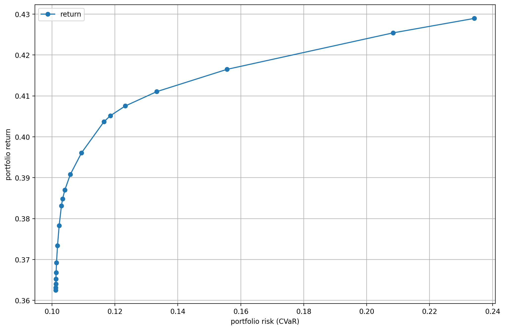
Fig. 8.1 The CVaR efficient frontier.

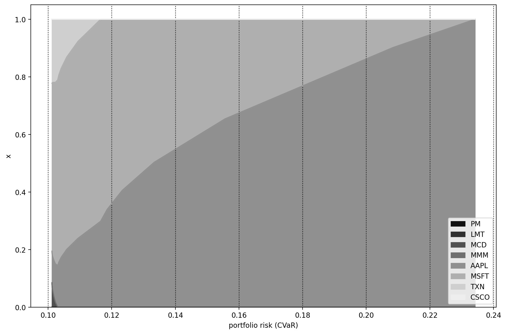
Fig. 8.2 Portfolio composition $\mathbf{x}$ with varying level of CVaR risk.

Footnotes

[1]

Tail dependence between two random variables means that their correlation is greater for more extreme events. Typical in financial markets, where extreme events are likely to happen together for multiple securities.

[2]

VaR only becomes coherent when return is normally distributed, but in this case it is proportional to the standard deviation.