4 Dealing with estimation error

As we have seen in Sec. 2 (Markowitz portfolio optimization), Markowitz portfolio optimization is a convenient and useful framework. However, in practice there is one important limitation [MM08]. The optimal solution is extremely sensitive to changes in the vector \(\EMean\) of estimated expected returns and the estimated covariance matrix \(\ECov\). Small changes in these input parameters often result in large changes in the optimal portfolio. The optimization basically magnifies the impact of estimation errors, yielding unintuitive, questionable portfolios and extremely small or large positions, which are difficult to implement. The instability causes unwarranted turnover and transaction costs.

It would help to use a larger estimation window, but the necessary amount of data grows unrealistically high quickly, because the size of the covariance matrix increases quadratically with the number of securities \(N\) [Bra10, CY16].

Fortunately there are multiple approaches to mitigating this issue. These can significantly reduce the impact of estimation errors and stabilize the optimization.

In the following we explore the main aspects of overcoming the estimation error issues.

4.1 Estimation of mean

The optimization is particularly sensitive to estimation errors in expected returns, small variations in sample means can lead to sizeable portfolio readjustments. Estimation based only on historical time-series can result in poor out-of-sample portfolio performance. Sample mean is hard to estimate accurately from historical data, because for all unbiased estimators the standard error fundamentally depends on the length (duration) of the time-series [Dod12]. Therefore to get better accuracy it is necessary to extend the time horizon, which is often problematic because data from a longer time interval might contain more structural changes, i. e. lack stationarity in its underlying parameters.

Despite these difficulties, the below methods offer an improvement on mean estimation.

4.1.1 Black-Litterman model

One way to deal with estimation error is to combine noisy data with prior information. We can base prior beliefs on recent regulatory, political and socioeconomic events, macroeconomy news, financial statements, analyst ratings, asset pricing theories, insights about market dynamics, econometric forecasting methods, etc. [AZ10]

The Black-Litterman model considers the market equilibrium returns implied by CAPM as a prior estimate, then allows the investor to update this information with their own views on security returns. This way we do not need noisy historical data for estimation [Bra10, CJPT18].

Thus we assume the distribution of expected return \(\mu\) to be \(\mathcal{N}(\EMean_\mathrm{eq}, \mathbf{Q})\), where \(\EMean_\mathrm{eq}\) is the equilibrium return vector, and the covariance matrix \(\mathbf{Q}\) represents the investor’s confidence in the equilibrium return vector as a realistic estimate.

The investor’s views are then modeled by the equation \(\mathbf{B}\mu = \mathbf{q} + \varepsilon\), where \(\varepsilon \sim \mathcal{N}(\mathbf{0}, \mathbf{V})\). Each row of this equation represents a view in the form of a linear equation, allowing for both absolute and relative statements on one or more securities. The views are also uncertain, we can use the diagonal of \(\mathbf{V}\) to set the confidence in them, small variance meaning strong confidence in a view.

By combining the prior with the views using Bayes’s theorem we arrive at the estimate

(4.1)\[\EMean_\mathrm{BL} = \mathbf{M}\mathbf{q} + (\mathbf{I} - \mathbf{M}\mathbf{B})\pi,\]

where \(\mathbf{M} = \mathbf{Q}\mathbf{B}^\mathsf{T}(\mathbf{B}\mathbf{Q}\mathbf{B}^\mathsf{T} + \mathbf{V})^{-1}\).

The prior \(\EMean_\mathrm{eq}\) is implied by the solution \(\mathbf{x} = \frac{1}{\delta}\ECov^{-1}\EMean\) of problem (2.3), by assuming that \(\mathbf{x} = \mathbf{x}_\mathrm{mkt}\), i. e., weights according to market capitalization.

We can also understand the Black–Litterman model as an application of generalized least-squares to combine two information sources (e. g. historical data and exogeneous views) [Bra10, The71]. Assuming the sources are independent, we write them into one linear equation with block structure as

(4.2)\[\begin{split}\begin{pmatrix} \pi\\ \mathbf{q} \end{pmatrix} = \begin{pmatrix} \mathbf{I}\\ \mathbf{B} \end{pmatrix} \mu + \begin{pmatrix} \varepsilon_\pi\\ \varepsilon_\mathbf{q} \end{pmatrix},\end{split}\]

where \(\pi\) is the prior, \(\varepsilon_\pi \sim \mathcal{N}(0, \mathbf{Q})\), \(\varepsilon_\mathbf{q} \sim \mathcal{N}(0, \mathbf{V})\), \(\mathbf{Q}\) and \(\mathbf{V}\) nonsingular. The solution will be

(4.3)\[\EMean_\mathrm{GLS} = (\mathbf{Q}^{-1} + \mathbf{B}^\mathsf{T}\mathbf{V}^{-1}\mathbf{B})^{-1} (\mathbf{Q}^{-1} \pi + \mathbf{B}^\mathsf{T}\mathbf{V}^{-1} \mathbf{q}).\]

Substituting \(\pi = \EMean_\mathrm{eq}\) we get a different form of \(\EMean_\mathrm{BL}\). [1]

Because the Black-Litterman model gives an expected return vector relative to the market equilibrium return, the optimal portfolio will also be close to the market portfolio, meaning it should not contain extreme positions. A drawback of this method is that the exogeneous views are assumed independent of historical data, which can be difficult to satisfy in practice. The model is extended further in [BGP12] to views on volatility and market dynamics.

4.1.2 Shrinkage estimation

Sample estimators are unbiased, but perform well only in the limit case of an infinite number of observations. For small samples their variance is large. In contrast, constant estimators have no variance, but display large bias. Shrinkage estimators improve the sample estimator by adjusting (shrinking) the sample estimator towards a constant estimator, the shrinkage target, basically finding the optimal tradeoff between variance and bias.

Shrinkage can also be thought of as regularization or a form of empirical Bayes estimation. Also the shrinkage target has to be consistent with other prior information and optimization constraints.

1. James–Stein estimator:

   This is the most widely known shrinkage estimator for the estimation of mean vector of a normal random variable with known covariance [EM76, LC98, Ric99]. The sample mean \(\EMean_\mathrm{sam}\) is normally distributed with mean \(\mu\) and covariance \(\Sigma/T\), where \(\Sigma\) is the covariance matrix of the data. Assuming \(\mathbf{b}\) as target, the James–Stein estimator will be

   \[\EMean_\mathrm{JS} = \mathbf{b} + (1-\alpha)(\EMean_\mathrm{sam} - \mathbf{b}),\]

   where the shrinkage coefficient is

   \[\alpha = \frac{1}{T}\frac{\tilde{N} - 2}{(\EMean_\mathrm{sam} - \mathbf{b})^\mathsf{T} \Sigma^{-1} (\EMean_\mathrm{sam} - \mathbf{b})},\]

   and \(\tilde{N} = \mathrm{Tr}(\Sigma)/\lambda_\mathrm{max}(\Sigma)\) is the effective dimension. The estimator improves \(\EMean_\mathrm{sam}\) for \(\tilde{N} > 2\), i. e., when \(\Sigma/T\) has not too different eigenvalues. Otherwise an estimator with coordinatewise different shrinkage coefficient is preferable, such as the one in [EM75].

   The target \(\mathbf{b}\) is arbitrary, but it is common to set it as the mean of means \(\mathbf{1}^\mathsf{T}\EMean_\mathrm{sam}/N\). This depends on the data, making the number of parameters to estimate one less, so the dimension \(\tilde{N}\) should be adjusted accordingly.

   We can further improve \(\EMean_\mathrm{JS}\) by the positive-part rule, when we set \((1-\alpha)\) to zero whenever it would be negative.

2. Jorion’s estimator [Jor86]:

   This estimator was derived in the context of portfolio analysis through an empirical Bayes approach. It uses the target \(b\mathbf{1}\), where \(b\) is the volatility-weighted mean of means:

   \[b = \frac{\mathbf{1}^\mathsf{T}\Sigma^{-1}\EMean_\mathrm{sam}}{\mathbf{1}^\mathsf{T}\Sigma^{-1}\mathbf{1}}.\]

   The shrinkage coefficient in this case is

   \[\alpha = \frac{N + 2}{N + 2 + T(\EMean_\mathrm{sam} - b\mathbf{1})^\mathsf{T} \Sigma^{-1} (\EMean_\mathrm{sam}- b\mathbf{1})}.\]

   If \(\Sigma\) is not known, it can be replaced by \(\frac{T-1}{T-N-2}\ECov\), where \(\ECov\) is the sample covariance matrix. The assumption of normality is not critical, but it gives more improvement over \(\EMean_\mathrm{sam}\) in “symmetric” situations, where variances are similar across data series.

4.2 Estimation of the covariance matrix

In contrast to the estimation of the mean, the standard error of the sample variance depends only on the sample size, making it possible to estimate from higher frequency data. Still, if the number of securities is high relative to the number of samples, the optimal solution can suffer from two issues [MM08]:

• Ill conditioning: We need to have sufficient amount of data to get a well-conditioned covariance estimate. A rule of thumb is that the number of observations \(T\) should be an order of magnitude greater than the number of securities \(N\).

• Estimation error: The estimation error of the covariance matrix increases quadratically (in contrast to linear increase in the case of the mean), so if \(N/T\) is large it can quickly become the dominant contributing factor to loss of accuracy.

When \(N/T\) is too large, the following regularization methods can offer an improvement over the sample covariance matrix [CM13]. Moreover, we can also apply factor models in this context, we discuss this in more detail in Sec. 5 (Factor models).

4.2.1 Covariance shrinkage

The idea is the same as in Sec. 4.1.2 (Shrinkage estimation), we try to achieve a balanced bias–variance tradeoff by shrinking the sample covariance matrix towards a shrinkage target. We can choose the latter in many ways, but it is important to be consistent with other prior information, e. g. what is implied by constraints.

The most well known shrinkage estimator is by Ledoit and Wolf; see [LW03a, LW03b, LW04] and [CM13] for a quick review. It combines the sample covariance matrix \(\ECov_\mathrm{sam}\) with the target \(\mathbf{B}\):

(4.4)\[\ECov_\mathrm{LW} = (1-\alpha)\ECov_\mathrm{sam} + \alpha\mathbf{B}.\]

We have to estimate the shrinkage intensity parameter \(\alpha\) depending on the target \(\mathbf{B}\). In practice it is also truncated so that \(\alpha \in [0, 1]\). Ledoit and Wolf propose three type of targets:

• Multiple of the identity matrix:

  (4.5)\[\mathbf{B}_\mathrm{I} = \bar{s}^2 \mathbf{I},\]

  where \(\bar{s}^2\) is the average sample variance. This target is optimal among all targets of the form \(c\mathbf{I}\) with \(c\in\mathbb{R}\). The corresponding optimal \(\alpha\) is

  \[\alpha = \frac{\frac{1}{T^2}\sum_{k=1}^T\mathrm{Tr}\left(\left[\mathbf{z}_k\mathbf{z}_k^\mathsf{T}-\ECov_\mathrm{sam}\right]^2\right)}{\mathrm{Tr}\left(\left[\ECov_\mathrm{sam}-\mathbf{B}_\mathrm{I}\right]^2\right)},\]

  where \(\mathbf{z}_k\) is observation \(k\) of the centered data matrix \(\mathbf{Z}\). See the details in [LW04].

  The sample covariance matrix \(\ECov_\mathrm{sam}\) can be ill-conditioned because estimation tends to scatter the sample eigenvalues further away from the mean \(\bar{\sigma}^2\) of the true unknown eigenvalues. This raises the condition number of \(\ECov_\mathrm{sam}\) relative to the true matrix \(\Sigma\) and this effect is stronger as the condition number of \(\Sigma\) is better or as \(N/T\) grows.

  The above shrinkage estimator basically pulls all sample eigenvalues back towards their grand mean \(\bar{s}^2\), the estimate of \(\bar{\sigma}^2\), thus stabilizing the matrix. We can also see this as a form of regularization.

• Single factor covariance matrices implied by the CAPM [2]:

  (4.6)\[\mathbf{B}_\mathrm{CAPM} = s_\mathrm{mkt}^2\beta\beta^\mathsf{T} + \ECov_\varepsilon,\]

  where \(s_\mathrm{mkt}^2\) is the sample variance of market returns, \(\beta\) is the vector of factor exposures, and \(\ECov_\varepsilon\) is the diagonal matrix containing the variances of the residuals. The single factor model is discussed in Sec. 5 (Factor models). In practice a proxy of the market factor could be the equally-weighted or the market capitalization-weighted portfolio of the constituents of a market index, resulting in two different shrinkage targets. The optimal shrinkage intensity is derived in [LW03b].

• Constant correlation covariance matrix:

  (4.7)\[\mathbf{B}_\mathrm{CC} = \bar{r}\sqrt{\mathbf{s}}\sqrt{\mathbf{s}}^\mathsf{T} + (1-\bar{r})\mathrm{Diag}(\mathbf{s}),\]

  where \(\mathbf{s} = \mathrm{diag}(\ECov_\mathrm{sam})\), and \(\bar{r} = \frac{2}{n(n-1)}\sum_{i=1}^{n-1}\sum_{j=i+1}^n r_{i, j}\) is the average sample correlation. The optimal shrinkage intensity is derived in [LW03a].

Notice that all three targets are positive definite matrices. Shrinkage towards a positive target guarantees that the resulting estimate is also positive, even when the sample covariance matrix itself is singular. Further advantage of this estimator is that it works also in the case of singular covariance matrices, when \(N>T\).

In [LW20], the authors present a nonlinear version of this estimator, which can apply different shrinkage intensity to each sample eigenvalue, resulting in even better performance.

4.2.2 Covariance de-noising

According to [dP19], the shrinkage method in Sec. 4.2.1 (Covariance shrinkage) does not discriminate between the eigenvalues associated with noise and the eigenvalues associated with signal, thus it weakens the signal as well. With the help of random matrix theory the method discussed here shrinks only the part of the covariance matrix that is associated with noise. Taking the covariance matrix \(\ECov\) it consists of the following steps:

1. Compute the correlation matrix from the covariance matrix: \(\mathbf{C} = \mathbf{D}^{-1/2}\ECov\mathbf{D}^{-1/2}\), where \(\mathbf{D} = \mathrm{Diag}(\ECov)\).

2. Compute the eigendecomposition of \(\mathbf{C}\) and compute the empirical distribution of the eigenvalues using Kernel Density Estimation.

3. Fit the Marčenko–Pastur distribution to the empirical distribution, which gives the theoretical bounds \(\lambda_+\) and \(\lambda_-\) on the eigenvalues associated with noise. This way we separate the spectrum into a random matrix (noise) component and the signal component. The eigenvalues of the latter will be above the theoretical upper bound \(\lambda_+\).

4. Change the eigenvalues below \(\lambda_+\) to their average, arriving at the de-noised correlation matrix \(\tilde{\mathbf{C}}\).

5. Recover the de-noised covariance matrix: \(\tilde{\ECov} = \mathbf{D}^{1/2}\tilde{\mathbf{C}}\mathbf{D}^{1/2}\).

4.2.3 Robust estimation

The reason for estimation error is partly that maximum likelihood estimators are highly sensitive to deviations from the assumed (typically normal) distribution. The empirical distribution of security returns usually deviates from the normal distribution [VD09]. Therefore it can be helpful to use robust estimation methods in the construction of mean-variance portfolios. Robust estimators are not as efficient as the maximum likelihood estimator but are stable even when the underlying model is not perfectly satisfied by the available data.

There are two approaches to involve robust statistics in portfolio selection:

• One-step methods: We perform the robust estimation and the portfolio optimization in a single step. We substitute the portfolio risk and portfolio return expressions by their robust counterparts. See for example in [VD09]. We discuss some examples in section Sec. 8 (Other risk measures).

• Two-step methods: First we compute the robust estimates of the mean vector and the covariance matrix of the data. This is followed by solving the usual portfolio optimization problem with the parameters replaced by their robust estimates. There are various robust covariance estimators, such as Minimum Covariance Determinant (MCD), 2D Winsorization, S-estimators. See for example in [RSTF20, WZ07]. We do not cover this topic in detail in this book.

4.3 Using constraints

Solutions from unconstrained portfolio optimization – while having elegant analytical formulas – can be unreliable in practice. The optimization can significantly overweight securities with large estimated returns, negative correlations, and small variances. The securities with the largest estimation error will get the largest positions. There will also be many zero positions, contradicting diversification [AZ10, MM08].

Financially meaningful constraints on the portfolio weights can also act as regularization, reducing error in the optimal portfolio [CM13]. In [DGNU09], \(L_1\) and \(L_2\) norm constraints are introduced for this purpose:

(4.8)\[\begin{split}\begin{array}{lrcl} \mbox{maximize} & \EMean^\mathsf{T}\mathbf{x} - \frac{\delta}{2} \mathbf{x}^\mathsf{T}\ECov\mathbf{x} & &\\ \mbox{subject to} & \mathbf{1}^\mathsf{T}\mathbf{x} & = & 1,\\ & \|\mathbf{x}\|_p^p & \leq & c.\\ \end{array}\end{split}\]

If \(p=1\) and \(c=1\) we get back the constraint \(\mathbf{x} \geq 0\), which prevents short-selling. In [JM03] the authors found that preventing short-selling or limiting position size is equivalent to shrinking all covariances of securities for which the respective constraint is binding. The short-selling constraint also implies shrinkage effect on the mean vector toward zero. In a conic optimization problem, the 1-norm constraint can be modeled based on Sec. 13.1.1.6 (Manhattan norm (1-norm)).

For the case \(p=1\) and \(c>1\) with the constraint \(\mathbf{1}^\mathsf{T}\mathbf{x} = 1\) also present, we get a “short-sale budget”, meaning that the total weight of short positions will be bounded by \((c-1)/2\). This allows the possibility of optimizing e. g. 130/30 type portfolios with \(c = 1.6\).

If \(p=2\) and the only constraint is \(\mathbf{1}^\mathsf{T}\mathbf{x} = 1\), then the minimum feasible value of \(c\) is \(1/N\), giving the \(\mathbf{x} = \mathbf{1}/N\) portfolio as the only possible solution. With larger values of \(c\) we get an effect equivalent to the Ledoit–Wolf shrinkage towards multiple of the identity. For other shrinkage targets \(\mathbf{B}\), the corresponding constraint will be \(\mathbf{x}^\mathsf{T}\mathbf{B}\mathbf{x} \leq c\) or \(\|\mathbf{G}^\mathsf{T}\mathbf{x}\|_2^2 \leq c\) where \(\mathbf{G}\mathbf{G}^\mathsf{T} = \mathbf{B}\). In a conic optimization problem, we can model the 2-norm constraint based on Sec. 13.1.1.7 (Euclidean norm (2-norm)).

In general,

• adding an \(L_1\) norm-constraint is equivalent to shrinking all covariances of securities that are being sold short. Instead of the elementwise short-sale constraints here we impose a global short-sale budget using only one constraint. This means that the implied shrinkage coefficient will be the same for all securities. According to the usual behavior of LASSO regression, the \(L_1\) norm-constrained portfolios are likely to assign a zero weight to at least some of the securities. This could be beneficial if we wish to invest only into a small number of securities.

• adding an \(L_2\) norm-constraint is equivalent to shrinking the sample covariance matrix towards the identity matrix. According to properties of ridge regression, the \(L_2\) norm-constrained portfolios will typically have a non-zero weight for all securities, which is good if we want full diversification.

4.4 Improve the optimization

In dealing with estimation error it is also a possibility to directly improve the optimization procedure.

4.4.1 Resampled portfolio optimization

To overcome estimation uncertainty we can use nonparametric bootstrap resampling on the available historical return data. This way we can create multiple instances of the data and generate multiple expected return and covariance matrix estimates using any estimation procedure. Then we compute the efficient frontier from all of them. Finally, we average the obtained solutions to make the effect of the estimation errors cancel out. This procedure is thoroughly analysed in [MM08].

Note that we should not average over portfolios of too different variances. Thus the averaging procedure assumes that for each pair of inputs we generate \(m\) points on the efficient frontier, and rank them \(1\) to \(m\). Then the portfolios with the same rank will be averaged.

In this process we can treat the number of simulated return samples in each batch of resampled data as a parameter. It can be used to measure the level of certainty of the expected return estimate. A large number of simulated returns is consistent with more certainty, while a small number is consistent with less certainty.

While this method offers good results in terms of diversification and mitigating the effects of estimation error, it has to be noted that it does this at the cost of intensive computational work.

According to [MM08], improving the optimization procedure is more beneficial than to use improved estimates (e. g. shrinkage) as input parameter. However, the two approaches do not exclude each other, so they can be used simultaneously.

4.4.2 Nested Clustering Optimization (NCO)

A recent method to tackle estimation error and error sensitivity of the optimization is described in [dP19]. The NCO method is capable of controlling for noise in the inputs, and also for instabilities arising from the covariance structure:

• Noise can arise from lack of data. As \(N/T\) approaches \(1\), the number of data points will approach the number of degrees of freedom in covariance estimation. Also based on random matrix theory, the smallest eigenvalue of the covariance matrix will be close to zero, raising the condition number.

• Instability in the optimal solution comes from the correlation structure, the existence of highly correlating clusters of securities. These will also raise the condition number of the covariance matrix. The most favorable correlation structure is that of the identity matrix.

The steps of NCO are the following:

1. Cluster the securities into highly-correlated groups based on the correlation matrix to get a partition \(P\) of the security universe. We could apply hierarchical clustering methods, or the method recommended in [dPL19]. It could be worthwhile to do the clustering also on the absolute value of the correlation matrix to see if it works better.

2. Run portfolio optimization for each cluster separately. Let \(\mathbf{x}_k\) denote the \(N\)-dimensional optimal weight vector of cluster \(P_k\), such that \(x_{k,i} = 0,\ \forall i \notin P_k\).

3. Reduce the original covariance matrix \(\ECov\) into a covariance matrix \(\ECov^\mathrm{cl}\) between clusters: \(\ECov^\mathrm{cl}_{k,l} = \mathbf{x}_k^\mathsf{T}\ECov\mathbf{x}_l\). The correlation matrix computed from \(\ECov^\mathrm{cl}\) will be closer to identity, making the inter-cluster optimization more accurate.

4. Run the inter-cluster portfolio optimization by treating each cluster as one security and using the reduced covariance matrix \(\ECov^\mathrm{cl}\). We will denote the resulting \(k\)-dimensional optimal weight vector by \(\mathbf{x}^\mathrm{cl}\).

5. Generate the final optimal portfolio: \(\mathbf{x} = \sum_k x^\mathrm{cl}_k\mathbf{x}_k\).

By splitting the problem in the above way into two independent parts, the error caused by intra-cluster noise cannot propagate across clusters.

In the paper the author also proposes a method for estimating the error in the optimal portfolio weights. We can use it with any optimization method, and facilitates comparison of methods in practice. The steps of this procedure can be found in Sec. 13.4 (Monte Carlo Optimization Selection (MCOS)).

4.5 Example

In this part we add shrinkage estimation to the case study introduced in the previous chapters. We start at the point where the expected weekly logarithmic returns and their covariance matrix is available:

return_array = df_weekly_log_returns.to_numpy()
m_weekly_log = np.mean(return_array, axis=0)
S_weekly_log = np.cov(return_array.transpose())

The eigenvalues of the covariance matrix are 1e-3 * [0.2993, 0.3996, 0.4156, 0.5468, 0.6499, 0.9179, 1.0834, 4.7805]. We apply the Ledoit–Wolf shrinkage with target (4.5):

N = S_weekly_log.shape[0]
T = return_array.shape[0]

# Ledoit--Wolf shrinkage
S = S_weekly_log
s2_avg = np.trace(S) / N
B = s2_avg * np.eye(N)
Z = return_array.T - m_weekly_log[:, np.newaxis]
alpha_num = alpha_numerator(Z, S)
alpha_den = np.trace((S - B) @ (S - B))
alpha = alpha_num / alpha_den
S_shrunk = (1 - alpha) * S + alpha * B

The function alpha_numerator is to compute the sum in the numerator of \(\alpha\):

def alpha_numerator(Z, S):
    s = 0
    T = Z.shape[1]
    for k in range(T):
        z = Z[:, k][:, np.newaxis]
        X = z @ z.T - S
        s += np.trace(X @ X)
    s /= (T**2)
    return s

In this example, we get \(\alpha=0.0843\), and the eigenvalues will become 1e-3 * [0.3699, 0.4618, 0.4764, 0.5965, 0.6909, 0.9363, 1.0879, 4.4732], closer to their sample mean as expected.

Next we implement the James–Stein estimator for the expected return vector:

# James--Stein estimator
m = m_weekly_log[:, np.newaxis]
o = np.ones(N)[:, np.newaxis]
S = S_shrunk
iS = np.linalg.inv(S)
b = (o.T @ m / N) * o
N_eff = np.trace(S) / np.max(np.linalg.eigvalsh(S))
alpha_num = max(N_eff - 3, 0)
alpha_den = T * (m - b).T @ iS @ (m - b)
alpha = alpha_num / alpha_den
m_shrunk = b + max(1 - alpha, 0) * (m - b)
m_shrunk = m_shrunk[:, 0]

In this case though it turns out that the effective dimension \(\tilde{N}\) would be too low for the estimator to give an improvement over the sample mean. This is because the eigenvalues of the covariance matrix are spread out too much, meaning that the uncertainty of the mean vector is primarily along the direction of one or two eigenvectors, effectively reducing the dimensionality of the estimation.

We can check the improvement on the plot of the efficient frontier Fig. 4.2. We can observe the portfolio composition for different risk-aversion levels on Fig. 4.2.

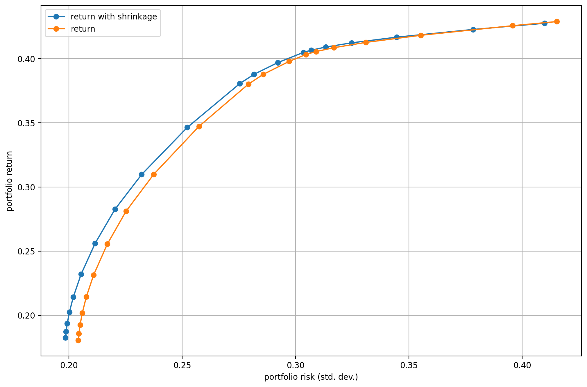
Fig. 4.1 The efficient frontier.

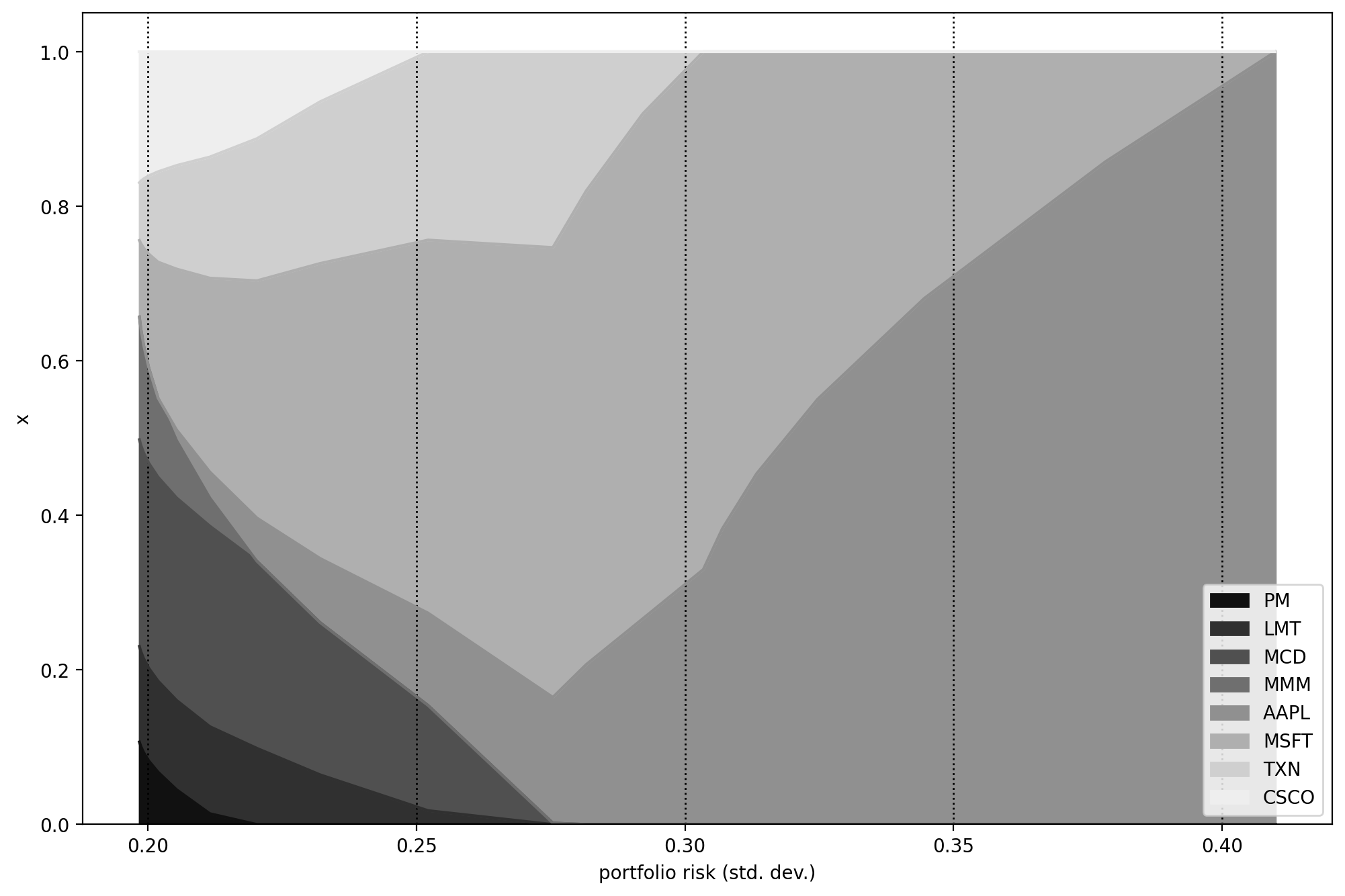
Fig. 4.2 Portfolio composition \(\mathbf{x}\) with varying level if risk-aversion \(\delta\).

Footnotes

[1]

We can derive this using \((\mathbf{A} + \mathbf{B})^{-1} = \mathbf{A}^{-1} - \mathbf{A}^{-1} \mathbf{B} (\mathbf{A} + \mathbf{B})^{-1}\) for nonsingular matrices.

[2]

The Capital Asset Pricing Model (CAPM) relates the expected return of securities (particularly stocks) to their systematic risk. We can calculate it as \(\mathbb{E}(R_i) = r^\mathrm{f} + \beta_i(\mathbb{E}(R_\mathrm{mkt}) - r^\mathrm{f})\), where \(\mathbb{E}(R_i)\) is the expected return, \(R^\mathrm{f}\) is the risk-free rate, \(\beta_i\) is the measure of systematic risk, and \(\mathbb{E}(R_\mathrm{mkt})\) is the expected return of the market.