3 Input data preparation

In Sec. 2.1.1 (Solution of the mean–variance model) we mentioned that the expected return vector \(\mu\) and the covariance matrix \(\Sigma\) of the securities needs to be estimated. In this chapter we will discuss this topic through a more general approach.

Portfolio optimization problems are inherently stochastic because they contain uncertain forward-looking quantities, most often the return of securities \(R\). In the case of the basic mean–variance optimization problems (2.1)-(2.3) the simple form of the objective and constraint functions make it possible to isolate uncertainty from the decision variables and wrap it into the parameters. This allows us to separate stochastic optimization into parameter estimation and deterministic optimization steps.

In many cases, for instance those involving different risk measures, however, it is not possible to estimate the optimization inputs as a separate step. These objectives or constraints can be a non-trivial function of portfolio returns, and thus we have to explicitly model the randomness. See examples in Sec. 8 (Other risk measures). Therefore more generally our goal is to estimate the distribution of returns over the investment time period. The simplest way to do that is by using the concept of scenario.

3.1 Scenarios

A scenario is a possible realization \(\mathbf{z}_k\) of the \(N\) dimensional random vector \(Z\) of a quantity corresponding to a given time period [MWOS15]. Thus we can also see a set of scenarios as a discretization of the distribution of \(Z\).

We denote the number of scenarios by \(T\). The probability of scenario \(\mathbf{z}_k\) occurring will be \(p_k\), with \(\sum_{k=1}^T p_k = 1\). In practice when the scenarios come from historical data or are obtained via computer simulation, all scenarios are assumed to have the same probability \(1/T\).

We commonly work with scenarios of the security returns \(R\). Scenario \(k\) of security returns will be \(\mathrm{r}_k\). Assuming that \(p_k = 1/T\), we can arrange the scenarios as columns of the \(N\times T\) matrix \(\mathbf{R}\).

Models involving certain risk measures can most easily be solved as convex optimization problems using scenarios (see Sec. 8 (Other risk measures)). This approach is called sample average approximation in stochastic optimization.

3.1.1 Scenario generation

Both the quality and the quantity of scenarios is important to get reliable optimal portfolios. Scenarios must be representative and also there must be enough of them to accurately model a random variable. Too few scenarios could lead to approximation errors, while too many scenarios could result in excessive computational cost. Next we discuss some common ways of generating scenarios.

3.1.2 Historical data

If we can assume that past realizations of a random quantity represents possible future outcomes, we can simply use historical data to create scenarios. Observations are then collected from a predetermined time window, with a given frequency. Each scenario would correspond to a vector of simultaneous observations for all \(N\) securities.

Using historical data is a simple non-parametric approach, but it could be inaccurate or insufficient in some cases:

• The underlying assumption about past realizations representing the future might not be realistic, if markets fundamentally change in the observed time period, or unexpected extreme events happen. Such changes can happen at least in every several years, often making the collection of enough representative historical data impossible.

• It can represent the tails of the distribution inaccurately because of low number of samples corresponding to the low probability tail events. Also these extreme values can highly depend on the given historical sample, and can fluctuate a lot when the sample changes.

• It depends on the observations being independent and identically distributed. Without this assumption, for example if the data exhibits autocorrelation, volatility clustering, etc., the distribution estimated based on historical scenarios will be inaccurate.

3.1.3 Monte Carlo simulation

With this approach we can generate a large number of scenarios according to a specified distribution. It can be useful in cases when there is a lack of historical scenarios available in the desired timeframe, but we have a model of the relevant probability distribution. This allows us to generate scenarios through a parametric approach. It has the following steps:

1. Select a (multivariate) probability distribution that explains all interesting features of the quantity of interest, e. g. fat tails and tail-dependence of return.

2. Estimate the distribution parameters using historical (independent and identically distributed) data samples.

3. Generate scenarios by sampling from the fitted distribution.

Later we will see an example of Monte Carlo scenario generation in Sec. 5.5.1 (Single factor model).

3.1.4 Performance assessment

We advise to have two separate sets of scenario data.

• The first one is the in-sample data, which we use for running the optimization and building the portfolio. We assume it known at the time of portfolio construction.

• The other data set is the out-of-sample data, which is for assessing the performance of the optimal portfolio. Out-of sample data is assumed to become available after the portfolio has been built.

3.2 Modeling the distribution of returns

In this section we describe how to estimate the distribution of security return over the time period of investment. It can be in the form of the estimated expected return and covariance matrix of securities, or in the form of a set of return scenarios.

The simplest case is when we have sufficient amount of return data for the desired time period, then we can estimate their distribution easily and proceed with the optimization. However, such data is seldom available, especially if the time period is very long, for reasons mentioned in Sec. 3.1.2 (Historical data). Therefore often we need to use higher frequency (shorter timeframe) data to estimate the distribution, then project the distribution to the longer timeframe of interest. This is typically not straightforward to do. We will describe this procedure first for stocks, then also outline the general method for other securities.

3.2.1 Notions of return

There are two different notions of return. Let \(P_{t_0}\) and \(P_{t_1}\) be the prices of a security at the beginning and end of a time period.

3.2.1.1 Linear return

Also called simple return, calculated as

\[R^\mathrm{lin} = \frac{P_{t_1}}{P_{t_0}}-1.\]

This return definition is the one we used so far in this book, the return whose distribution we would like to compute over the time period of investment.

We can aggregate linear returns across securities, meaning that the linear return of a portfolio is the average of the linear returns of its components:

(3.1)\[R^\mathrm{lin}_\mathbf{x} = \sum_i x_iR^\mathrm{lin}_i.\]

This is a property we need to be able to validly compute portfolio return and portfolio risk. However, it is not easy to scale linear return from one time period to another, for example to compute monthly return from daily return.

3.2.1.2 Logarithmic return

Also called continuously compounded return, calculated as

\[R^\mathrm{log} = \mathrm{log}\left(\frac{P_{t_1}}{P_{t_0}}\right).\]

We can aggregate logarithmic returns across time, meaning that the total logarithmic return over \(K\) time periods is the sum of all \(K\) single-period logarithmic returns: \(R^\mathrm{log}_K = \mathrm{log}\left(P_{t_K}/P_{t_0}\right) = \sum_{k=1}^{K} \mathrm{log}\left(P_{t_k}/P_{t_{k-1}}\right)\). This property makes it very easy to scale logarithmic return from one time period to another. However, we cannot average logarithmic returns the same way as linear returns, therefore they are unsuitable for computation of portfolio return and portfolio risk.

3.2.1.3 Relationship between returns

The two notions of return are related by

(3.2)\[R^\mathrm{log} = \mathrm{log}\left(1+R^\mathrm{lin}\right).\]

We must not confuse them, especially on longer investment time periods [Meu10a]. Logarithmic returns are suitable for projecting from shorter to longer time periods, while linear returns are suitable for computing portfolio level quantities.

3.2.2 Data preparation for stocks

Because both returns have properties necessary for portfolio optimization, the data preparation procedure for a stock portfolio is the following:

1. We start with logarithmic return data over the time period of estimation (e. g. one day if the data has daily frequency).

2. We estimate the distribution of logarithmic returns on this time period. If we assume that logarithmic returns are normally distributed, then here we estimate their mean vector and covariance matrix.

3. Using the property of aggregation across time we scale this distribution to the time period of investment (e. g. one year). We can scale the mean and covariance of logarithmic returns by the “square-root rule” [1]. This means that if \(h\) is the time period of investment and \(\tau\) is the time period of estimation, then

   \[\EMean_h = \frac{h}{\tau}\EMean_\tau,\quad \ECov_h = \frac{h}{\tau}\ECov_\tau.\]

4. Finally, we convert it into a distribution of linear returns over the period of investment. Then we can use the property of cross-sectional aggregation to compute portfolio return and portfolio risk. We show an example working with the assumption of normal distribution for logarithmic returns in Sec. 3.4 (Example).

3.2.3 Data preparation in general

We can generalize the above procedure to other types of securities; see in detail in [Meu05]. The role of the logarithmic return in case of stocks is generalized by the concept of market invariant. A market invariant is a quantity that determines the security price and is repeating (approximately) identically across time. Thus we can model it as a sequence of independent and identically distributed random variables. The steps will be the following:

1. Identify the market invariants. As we have seen, the invariant for the stock market is the logarithmic return. However, for other markets it is not necessarily the return, e. g. for the fixed-income market the invariant is the change in yield to maturity.

2. Estimate the joint distribution of the market invariant over the time period of estimation. Apart from historical data on the invariants, any additional information can be used. We can use parametric assumptions, approximate through moments, apply factor models, shrinkage estimators, etc., or simply use the empirical distribution, i. e., a set of scenarios.

3. Project the distribution of invariants to the time period of investment. Here we will assume that the invariants are additive across time, i. e., the invariant corresponding to a larger time interval is the sum of invariants corresponding to smaller intervals (the property that logarithmic returns have). Then the projection is easy to do through the characteristic function (see in [Meu05]), or we can also scale the moments by applying the “square-root rule” (see in [Meu10b]).

4. Map the distribution of invariants into the distribution of security prices at the investment horizon through a pricing function. Then compute the distribution of linear returns from the distribution of prices. If we have a set of scenarios, we can simply apply the pricing function on each of them.

This process will be followed in the case studies section in an example.

3.3 Extensions

In this section we discuss some use cases which need a more general definition of the MVO problem.

3.3.1 Generalization of linear return

While it is common to use linear return in portfolio optimization, it is not the most general approach. In certain cases we need to extend its definition to be able to do model the optimization problem [Meu10c]. As we have seen in Sec. 3.2.1 (Notions of return), the key property of linear return is the aggregation across securities (3.1). It allows us to define the expected portfolio return and the portfolio variance. We repeat the formula here in detail:

(3.3)\[R^\mathrm{lin}_\mathbf{x} = \frac{W_h - w_0}{w_0} = \sum_i \frac{v_i (P_{h,i} - p_{0,i})}{\mathbf{v}^\mathsf{T}\mathbf{p}_{0}} = \sum_i \frac{v_i p_{0,i}}{\sum_i v_i p_{0,i}} \frac{P_{h,i} - p_{0,i}}{p_{0,i}} = \sum_i x_i R^\mathrm{lin}_i,\]

where \(w_0 = \mathbf{v}^\mathsf{T}\mathbf{p}_0\) is the initial wealth, \(W_h = \mathbf{v}^\mathsf{T}P_h\) is the final wealth, \(\mathbf{v}\) is the vector of security holdings in terms of quantity, \(\mathbf{p}_0\) is the vector of initial security prices, and \(P_h\) is the vector of final security prices. We can see that maximizing linear return implicitly assumes that we wish to maximize final wealth.

Based on equation (3.3) there are two components in the aggregation formula that have to be well defined:

• Linear return of a security: It is given for security \(i\) as

  (3.4)\[R^\mathrm{lin}_i = \frac{P_{h,i} - p_{0,i}}{p_{0,i}}\]

  Linear return is not well defined if the price of the security \(p_{0,i}\) is zero. This can occur for example with swaps and futures.

• Portfolio weight: It is given for security \(i\) as

  (3.5)\[x_i = \frac{v_i p_{0,i}}{w_0}.\]

  Portfolio weight is not well defined if the initial wealth \(w_0\) (the total portfolio value at time \(t=0\)) is zero. This can occur for example in the case of dollar neutral long-short portfolios.

To be able to do portfolio optimization in the above mentioned special cases, we need to extend the definitions of portfolio weight and linear return such that we can apply the aggregation property (3.3).

• To extend the definition of linear return, we associate with each security a generalized normalizing quantity or basis \(b_i\) that takes the role of the security price \(p_{0,i}\) in the denominator of formula (3.4):

  (3.6)\[R^\mathrm{lin}_i = \frac{P_{h,i} - p_{0,i}}{b_i}\]

  The basis depends on the nature of the security; for swaps it can be the notional, for options it can be the strike or the underlying value, etc. It can be any value that results in an intuitive return definition to the portfolio manager. In most cases though it will be the price of the security, giving back the usual linear return definition (3.4).

• To extend the definition of the portfolio weight, we introduce a generalized portfolio basis \(b_\mathrm{P}\) that takes the role of the initial portfolio value \(w_0\) in the denominator of formula (3.5). We also use the relevant security basis \(b_i\) in the numerator:

  (3.7)\[x_i = \frac{v_ib_i}{b_\mathrm{P}}.\]

In general, the basis quantities \(b_i\ (i=1,\dots,N)\) and \(b_\mathrm{P}\) have to satisfy the following properties:

1. They are positive. This guarantees that for a long position, a positive net profit (P&L) will correspond to a positive return.

2. They are measured in the same money units as the P&L. This ensures that the return is dimensionless.

3. They are homogeneous, i.e. if \(b\) is the basis for one unit of security, then the basis for \(n\) unit of securities will be \(nb\). This ensures that the return is independent of the position size.

4. They are known at the beginning of the investment period (at time \(t=0\)). This ensures that the return will correspond to the full investment period.

By defining a basis value for each security and a basis value for the portfolio, computing the expected portfolio return and portfolio variance will be possible through the generalized aggregation formula:

(3.8)\[R^\mathrm{lin}_\mathbf{x} = \sum_i \frac{v_i b_i}{b_\mathrm{P}} \frac{P_{h,i} - p_{0,i}}{b_i} = \sum_i x_i R^\mathrm{lin}_i,\]

We can observe that in formula (3.8), the security level basis values \(b_i\) cancel out. This means that the value of the security level basis does not affect the portfolio return. It only matters in the context of interpreting the security weight and security return.

3.3.2 Portfolio scaling

During the introduction of the MVO problem in Sec. 2 (Markowitz portfolio optimization) we interpreted \(x_i\) as the fraction of wealth invested into security \(i\), such that the sum of weights is \(1\). This is, however, not the only possibility. From formula (3.8) we can see that the portfolio return and its interpretation or scaling is only affected by the portfolio level basis value \(b_\mathrm{P}\). We can select it independently of the security level basis values \(b_i\ (i=1,\dots,N)\), and thus change the scaling of the portfolio weights. Some natural choices:

• \(b_\mathrm{P} = \sum_i v_ib_i\). This choice ensures that the portfolio weights \(x_i\ (i=1,\dots,N)\) sum to \(1\), and thus represent fractions of \(b_\mathrm{P}\).

• \(b_\mathrm{P} = \sum_i v_ip_{0,i} = w_0\). In this case we normalize the P&L with the total portfolio value. For long only portfolio this is the same as the initial capital.

• \(b_\mathrm{P} = \sum_i |v_i|p_{0,i}\), the gross exposure. This provides an intuitive fraction interpretation to \(x_i\) for long-short portfolios as well.

• \(b_\mathrm{P} = C_\mathrm{init}\), the initial capital.

• \(b_\mathrm{P} = 1\). In this case formula (3.8) will become the total net profit (P&L) in dollars, and the portfolio weights will also be measured in dollars.

In this book, we will use \(b_\mathrm{P} = \sum_i v_ib_i\) by default. Any other choice will be explicitly stated.

3.3.3 Long-short portfolios

When working with a long-short portfolio, we also have to extend the MVO problem slightly. If the investor can short sell and also use leverage (e. g. margin loan), then the total value of the investment (the gross exposure) can be greater than the amount of initial capital. In case of leverage, the gross exposure provides better insight into the risks taken than the total capital, so being fully invested is no longer meaningful as a sole constraint.

Therefore in the optimization problem formulation of typical long-short portfolios, we will substitute the budget constraint (2.5) to a gross exposure limit, i. e., a leverage constraint:

\[\sum_{i} |v_i|p_{0,i} \leq L \cdot C_\mathrm{init},\]

where \(C_\mathrm{init}\) is the initial invested capital, and \(L\) is the leverage limit. If we normalize here with \(b_\mathrm{P} = C_\mathrm{init}\), then we get

\[\|\mathbf{x}\|_1 \leq L.\]

For example, Regulation-T states that for long positions the margin requirement is 50% of the position value, and for short positions the collateral requirement is 150% of the position value (of which 100% comes from short sale proceeds). This translates into \(L = 2\). A special case of \(L = 1\) would mean that we can short sell but have no leverage.

A more general version of the leverage constraint is

\[\sum_{i} m_i|x_i| \leq 1.\]

where \(m_i\) is the margin requirement of position \(i\). In case of Reg-T we had \(m_i = \frac{1}{2}\) for all \(i\).

We might also impose an enhanced active equity structure on the portfolio, like 120/20 or 130/30. This is typically considered when it is possible to use the short sale proceeds to purchase more securities (another form of leverage), so there is no need to use margin loans. Such a portfolio has 100% market exposure, which is expressed by

\[\sum_{i} v_ip_{0,i} = C_\mathrm{init},\]

or writing the same using \(\mathbf{x}\) after normalizing again with \(b_\mathrm{P} = C_\mathrm{init}\), we get the ususal budget constraint

\[\sum_i x_i = 1.\]

For example, 130/30 type portfolio would have the constraints \(\|\mathbf{x}\|_1 \leq 1.6\) and \(\mathbf{1}^\mathsf{T}\mathbf{x} = 1\).

We can also use factor neutrality constraints on a long-short portfolio. We can achieve this simply by adding a linear equality constraint expressing that the portfolio should be orthogonal to a vector \(\beta\) of factor exposures:

\[\beta^\mathsf{T}\mathbf{x} = 0.\]

A special case of this is when the factor exposures are all ones; then the portfolio will be dollar neutral:

\[\mathbf{1}^\mathsf{T}\mathbf{x} = 0.\]

We have to note that in the case of dollar neutrality, the total portfolio value is \(0\). Referring back to the discussion about portfolio weights in Sec. 3.3.1 (Generalization of linear return), in this case the portfolio weights cannot be defined as (3.5). Instead, we need to define a \(b_\mathrm{P}\) that is different from \(w_0\). See also in Sec. 3.3.2 (Portfolio scaling).

Note also that if we model using the quadratic cone instead of the rotated quadratic cone and \(\mathbf{x} = \mathbf{0}\) is a feasible solution, then there will be no optimal portfolios which are not fully invested. The solutions will be either \(\mathbf{x} = \mathbf{0}\) or some risky portfolio with \(\|\mathbf{x}\|_1 = 1\). See a detailed discussion about this in Sec. 13.3 (Quadratic cones and riskless solution).

3.4 Example

In this example we will show a case with real data, that demonstrates the steps in Sec. 3.2.3 (Data preparation in general) and leads to the expected return vector and the covariance matrix we have seen in Sec. 2.4 (Example).

3.4.1 Problem statement

Suppose that we wish to invest in the U.S. stock market with a long-only strategy. We have chosen a set of eight stocks and we plan to re-invest any dividends. We start to invest at time \(t=0\) and the time period of investment will be \(h=1\) year, ending at time \(t=1\).

We also have a pre-existing allocation \(\mathbf{v}_0\) measured in number of shares. We can express this allocation also in fractions of total dollar value \(\mathbf{v}_0^\mathsf{T}\mathbf{p}_0\), by \(\mathbf{x}_0 = \mathbf{v}_0 \circ \mathbf{p}_0 / \mathbf{v}_0^\mathsf{T}\mathbf{p}_0\).

Our goal is to derive a representation of the distribution of one year linear returns at time \(t=1\), and use it to solve the portfolio optimization problem. Here we will represent the distribution with the estimate \(\EMean\) of the expected one year linear returns \(\mu = \mathbb{E}(R)\) and with the estimate \(\ECov\) of the covariance of one year linear returns \(\Sigma = \mathrm{Cov}(R)\), at the time point \(t=1\).

3.4.2 Data collection

We obtain a time-series of daily stock prices from data providers, for a five year period (specifically from 2016-03-21 until 2021-03-18), adjusted for splits and dividends. During this time period the market was generally bullish, with only short downturn periods. This will be reflected in the estimated mean return vector and in the covariance structure. See a deeper analysis in Sec. 5.5.1 (Single factor model).

We choose an estimation time period of one week as a balance between having enough independent observations and the homogeneity of the data series. Thus \(\tau = 1/52\) year.

At this point we assume that the price data is available in the pandas DataFrame df_prices. The graphs of the price time-series can be seen on Fig. 3.1:

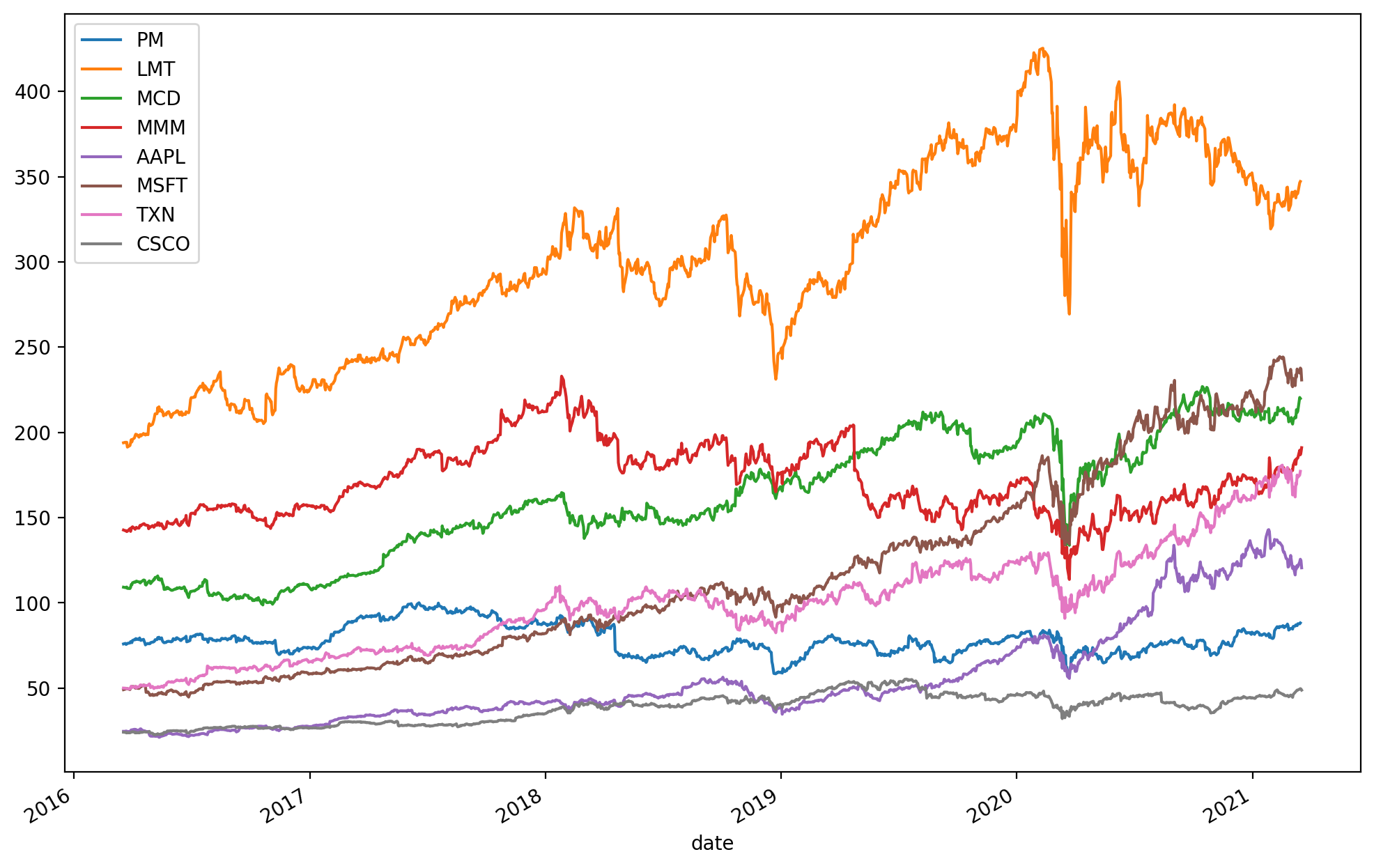
Fig. 3.1 Daily prices of the 8 stocks in the example portfolio.

3.4.3 Estimation of moments

Now we will go over the steps in Sec. 3.2.3 (Data preparation in general).

3.4.3.1 Market invariants

For stocks, both linear and logarithmic returns are market invariants, however it is easier to project logarithmic returns to longer time periods. It also has an approximately symmetrical distribution, which makes it easier to model. Therefore we resample each price time series to weekly frequency, and obtain a series of approximately 250 non-overlapping observations:

df_weekly_prices = df_prices.resample('W').last()

Next we compute weekly logarithmic returns from the weekly prices, followed by basic handling of missing values:

df_weekly_log_returns =
         np.log(df_weekly_prices) - np.log(df_weekly_prices.shift(1))
df_weekly_log_returns = df_weekly_log_returns.dropna(how='all')
df_weekly_log_returns = df_weekly_log_returns.fillna(0)

3.4.3.2 Distribution of invariants

To estimate the distribution of market invariants, in this example we choose a parametric approach and fit the weekly logarithmic returns to a multivariate normal distribution. This requires the estimation of the distribution parameters \(\mu_\tau^\mathrm{log}\) and \(\Sigma_\tau^\mathrm{log}\). For simplicity we use the sample statistics denoted by \(\EMean_\tau^\mathrm{log}\) and \(\ECov_\tau^\mathrm{log}\). The “log” superscript indicates that these statistics correspond to the logarithmic returns. In code this looks like

return_array = df_weekly_log_returns.to_numpy()
m_weekly_log = np.mean(return_array, axis=0)
S_weekly_log = np.cov(return_array.transpose())

3.4.3.3 Projection of invariants

We project the distribution of the weekly logarithmic returns represented by \(\EMean_\tau^\mathrm{log}\) and \(\ECov_\tau^\mathrm{log}\) to the one year investment horizon. Because the logarithmic returns are additive across time, the projected distribution will also be normal with parameters \(\EMean_h^\mathrm{log} = \frac{h}{\tau}\EMean_\tau^\mathrm{log}\) and \(\ECov_h^\mathrm{log} = \frac{h}{\tau}\ECov_\tau^\mathrm{log}\).

m_log = 52 * m_weekly_log
S_log = 52 * m_weekly_log

3.4.3.4 Distribution of linear returns

To obtain the distribution of linear returns at the investment horizon \(h\), we first derive the distribution of security prices at the investment horizon. Using the characteristic function of the normal distribution, and the pricing function \(P_h = \mathbf{p}_0\mathrm{exp}\left(R^\mathrm{log}\right)\), we get

(3.9)\[\begin{split}\begin{array}{lcr} \mathbb{E}(P_h) & = & \mathbf{p}_0 \circ \mathrm{exp}\left(\EMean_h^\mathrm{log} + \frac{1}{2}\mathrm{diag}(\ECov_h^\mathrm{log})\right), \\ \mathrm{Cov}(P_h) & = & \mathbb{E}(P_h)\mathbb{E}(P_h)^\mathsf{T} \circ (\mathrm{exp}(\ECov_h^\mathrm{log}) - 1). \end{array}\end{split}\]

In code, this will look like

p_0 = df_weekly_prices.iloc[0].to_numpy()
m_P = p_0 * np.exp(m_log + 1/2*np.diag(S_log))
S_P = np.outer(m_P, m_P) * (np.exp(S_log) - 1)

Then the estimated moments of the linear return is easy to get by \(\EMean = \frac{1}{\mathbf{p}_0} \circ \mathbb{E}(P_h) - \mathbf{1}\) and \(\ECov = \frac{1}{\mathbf{p}_0\mathbf{p}_0^\mathsf{T}} \circ \mathrm{Cov}(P_h)\), where \(\circ\) denotes the elementwise product and division by a vector or a matrix is also done elementwise.

m = 1 / p_0 * m_P - 1
S = 1 / np.outer(p_0, p_0) * S_P

Notice that we could have computed the distribution of linear returns from the distribution of logarithmic returns directly is this case, using the simple relationship (3.2). However in general for different securities, especially for derivatives we derive the distribution of linear returns from the distribution of prices. This case study is designed to demonstrate the general procedure. See details in [Meu05, Meu11].

Also in particular for stocks we could have started with linear returns as market invariants, and model their distribution. Projecting it to the investment horizon, however, would have been much more complicated. There exist no scaling formulas for the linear return distribution or its moments as simple as the ones for logarithmic returns.

Footnotes

[1]

Originally the square-root rule for stocks states that we can annualize the standard deviation \(\sigma_\tau\) of \(\tau\)-day logarithmic returns by \(\sigma_\mathrm{ann} = \sigma_\tau\sqrt{252/\tau}\), where \(\sigma_\mathrm{ann}\) is the annualized standard deviation, and \(252\) is the number of business days in a year.