5 Factor models

The purpose of factor models is to impose a structure on financial variables and their covariance matrix by explaining them through a small number of common factors. This can help to overcome estimation error by reducing the number of parameters, i. e., the dimensionality of the estimation problem, making portfolio optimization more robust against noise in the data. Factor models also provide a decomposition of financial risk to systematic and security specific components [CM13]. Factor models can be generalized in many ways; see in [BS11].

5.1 Definition

Let \(Z_t\) be an \(N\)-dimensional random vector representing a financial variable at time \(t\). We can write \(Z_t\) as a linear function of components as

\[Z_t = \beta F_t + \theta_t,\]

where \(F_t\) is a \(K\)-dimensional random vector representing the common factors at time \(t\), \(\beta\) is the \(N\times K\) matrix of factor exposures (or loadings, betas), and \(\theta_t = \alpha + \varepsilon_t\) is the specific component such that \(\mathbb{E}(\theta_t) = \alpha\) and \(\varepsilon_t\) is white noise [1] with covariance \(\Sigma_\theta\). If \(Z_t\) represents security returns, then \(\beta\mathbb{E}(F_t)\) is the expected explained return and \(\alpha\) is the expected unexplained return.

Factor models typically work with the following assumptions:

• Exact factor model: All common movement between pairs of variables is modeled by the factors. This means that the covariances of \(Z_t\) is determined only by the covariances of \(F_t\). This gives the conditions \(\mathrm{Cov}(\varepsilon_{t_1}, F_{t_2}) = \mathbf{0}\) for all \(t_1, t_2\) and that \(\mathrm{Cov}(\varepsilon_t) = \Sigma_\varepsilon\) is diagonal. [2]

• Static factor model: \(F_t\) only has a contemporaneous effect on \(Z_t\). [3]

• Weakly stationary factors: The sequence of random variables \(F_t\) are weakly stationary so that \(\mathbb{E}(F_t) = \mu_F\) and \(\mathrm{Cov}(F_t) = \Sigma_F\). This allows us to estimate the model from (historical) scenarios.

With these assumptions, we can write the expected value of \(Z_t\) as

\[\mu_Z = \alpha + \beta\mu_F.\]

The covariance matrix will be given by

\[\Sigma_Z = \beta\Sigma_F\beta^\mathsf{T} + \Sigma_\theta.\]

These two equations allow the following properties:

• Number of parameters: The covariance matrix \(\Sigma_Z\) has only \(NK + N + K(K+1)/2\) parameters, which is linear in \(N\), in contrast to having \(N(N+1)/2\) covariances, which is quadratic in \(N\).

• Risk decomposition: Because the common factors and the specific components are uncorrelated, we can separate the risks associated with each. For a portfolio \(\mathbf{x}\) the portfolio level factor exposures are given by \(\mathbf{b} = \beta^\mathsf{T}\mathbf{x}\) and we can write the total portfolio variance as \(\mathbf{b}^\mathsf{T}\Sigma_F\mathbf{b} + \mathbf{x}^\mathsf{T}\Sigma_\theta\mathbf{x}\).

• While the factor structure may introduce a bias on the covariance estimator, it will also lower its variance owing to the reduced number of parameters to estimate.

5.2 Classes of factor models

5.2.1 Explicit factor models

In these models the factors are predefined based on financial or economic theory, independently from the data. They are observed from e. g. macroeconomic quantities (inflation, economic growth, etc.) or from security characteristics (industry, dividend yield, market capitalization, etc.) [Con95]. The goal of these models is typically to explain security returns. A drawback of explicit factor models is the misspecification risk. The derivation of the covariance matrix \(\Sigma_Z\) strongly relies on the orthogonality between the factors \(F_t\) and the residuals \(\theta_t\), which might not be satisfied if relevant factors are missing from the model.

5.2.1.1 Macroeconomic models

In the case of macroeconomic factor models we observe the historical factor time-series \(\mathbf{F}\) and apply time-series regression to get estimators for \(\beta\), \(\alpha\), and \(\varepsilon\). However, enough stationary data must be available for an accurate regression.

The simplest macroeconomic factor models use a single factor as common risk component. In Sharpe’s single factor model this common factor is the market risk. In practice, we can approximate the market risk factor using the returns of a stock index, by either forming an equally-weighted or a market capitalization-weighted portfolio of the index constituents. The covariance matrix with single factor model structure has only \(2N+1\) parameters to estimate.

5.2.1.2 Fundamental models

There are two methods to estimate fundamental factor models:

• BARRA method: We compute the estimate \(\EBeta\) of the \(\beta\) from the observed security specific attributes (assumed to be time invariant). Then we do cross-sectional regression for each time instant \(t\) to obtain the factor time-series \(\mathbf{F}\) and its estimated covariance matrix \(\ECov_F\): \(\mathbf{F}_t = (\EBeta^\mathsf{T}\ECov_\theta^{-1}\EBeta)^{-1}\EBeta^\mathsf{T}\ECov_\theta^{-1}\mathbf{Z}_t\), where \(\ECov_\theta\) is the diagonal matrix of estimated specific variances. It is there to take into account cross-sectional heteroskedasticity in the model.

• Fama–French method: For each time \(t\) we order the securities into quintiles by a given security attribute. Then we long the the top quintile and short the bottom quintile. The factor realization at time \(t\) corresponding to the chosen attribute will be the return of this hedged portfolio. After obtaining the factor time-series corresponding to each attribute, we can estimate \(\beta\) using time-series regression.

5.2.2 Implicit factor models

Implicit factor models derive both the factors and the factor exposures from the data, so these does not need any external input. However, the statistical estimation procedures involved are prone to discovering spurious correlations, and they can only work if we assume the factor exposures to be time invariant over the estimation period. Also, implicit factors do not have financial interpretation. Mainly two methods are used to derive the factors.

5.2.2.1 Factor analysis

This method assumes a more specific structure, a normal factor model that has the additional requirements \(\mathbb{E}(F_t) = \mathbf{0}\) and \(\mathrm{Cov}(F_t) = \mathbf{I}\).

• To satisfy the first condition, we redefine \(\alpha' = \alpha + \beta\mathbb{E}(F_t)\).

• To satisfy the second condition, we observe that the variables \(\beta\) and \(\mathbf{F}_t\) can only be determined up to an invertible matrix \(\mathbf{H}\), because \(\beta\mathbf{F}_t = \beta\mathbf{H}^{-1}\mathbf{H}\mathbf{F}_t\). Thus we decompose the factor covariance as \(\Sigma_F = \mathbf{Q}\mathbf{Q}^\mathsf{T}\) and choose \(\mathbf{H} = \mathbf{Q}^{-1}\) to arrive at the desired structure.

The covariance matrix will then become \(\Sigma_Z = \beta\beta^\mathsf{T} + \Sigma_\theta\). The matrix \(\mathbf{Q}\) is still determined only up to a rotation. This freedom can help in finding interpretation for the factors.

Further assuming that the variables \(Z_t\) are independent and identically normally distributed, we can compute estimates \(\EAlpha\), \(\EBeta\), and \(\ECov_\theta\) using maximum likelihood method. Then we use cross-sectional regression to estimate the factor time-series: \(\mathbf{F}_t = (\EBeta^\mathsf{T}\ECov_\theta^{-1}\EBeta)^{-1}\EBeta^\mathsf{T}\ECov_\theta^{-1}(\mathbf{z}_t - \EAlpha)\). Here we used \(\ECov_\theta^{-1}\) as weighting to address cross-sectional heteroskedasticity in \(\varepsilon_t\).

The number of factors can be determined e. g. using likelihood ratio test. The drawback of factor analysis is that it is not efficient for large problems.

5.2.2.2 Principal Component Analysis

5.2.2.2.1 Definition

Principal component analysis (PCA) is an affine dimension reduction method. Let us define factors (called principal components) through \(F_t =\mathbf{d} + \mathbf{A} Z_t\), assuming \(\mathbb{E}(F_t) = \mathbf{0}\), and \(\mathrm{dim}(F_t) = K < N = \mathrm{dim}(Z_t)\). Then we can approximate \(Z_t\) with \(\tilde{Z}_t = \alpha + \beta F_t\). The best such approximation is obtained by the eigendecomposition \(\Sigma_Z = \mathbf{V}\Lambda\mathbf{V}^\mathsf{T}\), where the matrix \(\Lambda\) is diagonal with the eigenvalues \(\lambda_1,\dots,\lambda_N\) in it ordered from largest to smallest, and the matrix \(\mathbf{V}\) contains the corresponding eigenvectors \(\mathbf{v}_1,\dots,\mathbf{v}_N\) as columns.

If we partition the eigenvector matrix as \(\mathbf{V}=[\mathbf{V}_{K}, \mathbf{V}_{N-K}]\), where \(\mathbf{V}_{K}\) consists of the first \(K\) eigenvectors, we can construct the solution:

\[\begin{split}\begin{array}{rcl} \beta & = & \mathbf{V}_{K}, \\ \alpha & = & \mathbb{E}(Z_t), \\ \mathbf{F}_t & = & \mathbf{V}_{K}^\mathsf{T}(Z_t - \mathbb{E}(Z_t)), \\ \varepsilon_t & = & Z_t- \tilde{Z}_t = \mathbf{V}_{N-K}\mathbf{V}_{N-K}^\mathsf{T}(Z_t - \mathbb{E}(Z_t)). \end{array}\end{split}\]

Note that for \(\varepsilon_t\) we have \(\mathbb{E}(\varepsilon_t) = \mathbf{0}\) and \(\mathrm{Cov}(F_t, \varepsilon_t) = \mathbf{0}\), as required in the factor model definition. Also the factors will be uncorrelated: \(\Sigma_F = \frac{1}{T}F_tF_t^\mathsf{T} = \Lambda_K\), containing the first \(K\) eigenvalues in the diagonal.

Intuitively PCA does an orthogonal projection of \(Z_t\) onto the hyperplane spanned by the \(K\) directions corresponding to the \(K\) largest eigenvalues. This way the projection \(\tilde{Z}_t\) contains the most randomness of the original variable \(Z_t\) that an affine transformation can preserve. The eigenvalue \(\lambda_i\) measures the randomness of principal component \(F_{t,i}\), the randomness of \(Z_t\) along the direction \(\mathbf{v}_i\). The ratio \(\sum_{i=1}^K \lambda_i / \sum_{i=1}^N \lambda_i\) is the fraction of randomness explained by the factor model approximation.

Advantages of PCA based factor models is that they are computationally simple, they need no external data, and that they avoid misspecification risk because the residuals and the factors are orthogonal by construction. Also they yield factors ranked according to their fraction of explained variance, which can help determining the number of factors \(K\) to use.

5.2.2.2.2 Number of factors

In practice, the number of factors \(K\) is unknown and has to be estimated. Too few factors reduce the explanatory power of the model, too many could lead to retaining insignificant factors. In [BN01] the authors propose an information criteria to estimate \(K\):

\[K^* = \mathrm{argmin}_K \mathrm{log}\left(\varepsilon_K^T\varepsilon_K\right) + K\left(\frac{N+T}{NT}\right)\mathrm{log}\left(\frac{NT}{N+T}\right),\]

where \(\varepsilon_K\) is the vector of residuals in the case of \(K\) factors.

If we wish to keep the number of factors time invariant, then a heuristic method can help: \(K = \lfloor\mathrm{log}(N)\rfloor\).

5.2.2.2.3 PCA on the correlation matrix

We can also do PCA on the correlation matrix:

• We get the correlation matrix \(\Omega_Z\) from the covariance matrix \(\Sigma_Z\) by \(\Omega_Z = \mathbf{D}^{-1/2}\Sigma_Z\mathbf{D}^{-1/2}\), where \(\mathbf{D} = \mathrm{Diag}(\Sigma_Z)\).

• Then we keep only the \(K\) largest eigenvalues: \(\tilde{\Omega}_Z = \mathbf{V}_K\Lambda_K\mathbf{V}_K^\mathsf{T}\).

• To guarantee that this approximation will also be a correlation matrix, we add a diagonal correction term \(\mathrm{Diag}\left(\mathbf{I} - \tilde{\Omega}_Z\right)\).

• Finally, we transform the result back into a covariance matrix.

This method can give better performance when the scale of data variables is very different.

5.2.2.2.4 Practical considerations

In practice, PCA relies on the assumption that the number of observations \(T\) is large relative to the number of securities \(N\). If this does not hold, i. e., \(N > T\), then we can do PCA in a different way. Suppose that \(\mathbf{Z}\) is the \(N\times T\) data matrix, and \(\EMean\) is the mean of the data. Then

• We do eigendecomposition on the \(T\times T\) matrix \(\frac{1}{N}(\mathbf{Z} - \EMean\mathbf{1}^\mathsf{T})^\mathsf{T}(\mathbf{Z} - \EMean\mathbf{1}^\mathsf{T}) = \mathbf{W}\Lambda\mathbf{W}^\mathsf{T}\).

• We get the principal component matrix as \(\mathbf{F} = \Lambda\mathbf{W}^\mathsf{T}\).

The most efficient way to compute PCA is to use singular value decomposition (SVD) directly on the data matrix \(\mathbf{Z}\). Then we get \(\mathbf{Z} = \mathbf{V}\Lambda\mathbf{W}^\mathsf{T}\). Now it is easy to see the connection between the two PCA approaches:

\[\mathbf{F} = \mathbf{V}^\mathsf{T}\mathbf{Z} = \mathbf{V}^\mathsf{T}\mathbf{V}\Lambda\mathbf{W}^\mathsf{T} = \Lambda\mathbf{W}^\mathsf{T}.\]

5.3 Portfolio optimization with factor model

5.3.1 Sparsity

Suppose we have the decomposition of the covariance matrix \(\ECov_Z=\EBeta\ECov_F\EBeta^\mathsf{T}+\ECov_\theta\), where \(\ECov_F\) is the \(K\times K\) sample factor covariance matrix and \(K\) is the number of factors. Typically we have only a few factors, so \(K \ll N\) and thus \(\ECov_F\) is much lower dimensional than the \(N\times N\) matrix \(\ECov_Z\). This makes it much cheaper to find the decomposition \(\ECov_F=\mathbf{F}\mathbf{F}^\mathsf{T}\), and consequently the factorization \(\ECov_Z=\mathbf{G}\mathbf{G}^\mathsf{T}\), where

(5.1)\[\mathbf{G} = \begin{bmatrix} \EBeta\mathbf{F} & \ECov_\theta^{1/2} \end{bmatrix}.\]

This form of \(\mathbf{G}\) is typically very sparse. In practice sparsity is more important than the number of variables and constraints in determining the computational efficiency of the optimization problem. Thus it can be beneficial to focus on the number of nonzeros in the matrix \(\mathbf{G}\) and try to reduce it. Indeed, the \(N \times (N+K)\) dimensional \(\mathbf{G}\) is larger than the \(N\times N\) dimensional Cholesky factor of \(\ECov_Z\) would be, but in \(\mathbf{G}\) there are only \(N(K + 1)\) nonzeros in contrast to the \(N(N + 1)/2\) nonzeros in the Cholesky factor. Because in practice \(K\) tends to be a small number independent of \(N\), we can conclude that the usage of a factor model reduced the number of nonzeros, and thus the storage requirement by a factor of \(N\). This will in most cases also lead to a significant reduction in the solution time.

5.3.2 Modeling risk terms

In the risk minimization setting (2.1) of the Markowitz problem, according to Sec. 13.1.1.10 (Quadratic form) we can model the factor risk term \(\mathbf{x}^\mathsf{T}\EBeta\ECov_F\EBeta^\mathsf{T}\mathbf{x} \leq t_1\) as \((\frac{1}{2}, t_1, \mathbf{F}^\mathsf{T}\EBeta^\mathsf{T}\mathbf{x}) \in \mathcal{Q}^{K+2}\), and the specific risk term \(\mathbf{x}^\mathsf{T}\ECov_\theta\mathbf{x} \leq t_2\) as \((\frac{1}{2}, t_2, \ECov_\theta^{1/2}\mathbf{x}) \in \mathcal{Q}^{N+2}\). The latter can be written in a computationally more favorable way as \(\left(\frac{1}{2}, t_2, \mathrm{diag}\left(\ECov_\theta^{1/2}\right)\circ\mathbf{x}\right) \in \mathcal{Q}^{N+2}\). The resulting risk minimization problem will then look like

(5.2)\[\begin{split}\begin{array}{lrcl} \mbox{minimize} & t_1 + t_2 & &\\ \mbox{subject to} & (\frac{1}{2}, t_1, \mathbf{F}^\mathsf{T}\EBeta^\mathsf{T}\mathbf{x}) & \in & \mathcal{Q}_\mathrm{r}^{K+2},\\ & \left(\frac{1}{2}, t_2, \mathrm{diag}\left(\ECov_\theta^{1/2}\right)\circ\mathbf{x}\right) & \in & \mathcal{Q}_\mathrm{r}^{N+2},\\ & \EMean^\mathsf{T}\mathbf{x} & \geq & r_\mathrm{min},\\ & \mathbf{x} & \in & \mathcal{F}. \end{array}\end{split}\]

We can also have prespecified limits \(\gamma_1\) for the factor risk and \(\gamma_2\) for the specific risk. Then we can use the return maximization setting:

(5.3)\[\begin{split}\begin{array}{lrcl} \mbox{maximize} & \EMean^\mathsf{T}\mathbf{x} & &\\ \mbox{subject to} & (\frac{1}{2}, \gamma_1^2, \mathbf{F}^\mathsf{T}\EBeta^\mathsf{T}\mathbf{x}) & \in & \mathcal{Q}_\mathrm{r}^{K+2},\\ & \left(\frac{1}{2}, \gamma_2^2, \mathrm{diag}\left(\ECov_\theta^{1/2}\right)\circ\mathbf{x}\right) & \in & \mathcal{Q}_\mathrm{r}^{N+2},\\ & \mathbf{x} & \in & \mathcal{F}. \end{array}\end{split}\]

5.4 Shrinkage as factor model

In section Sec. 4.2.1 (Covariance shrinkage) we discussed that shrinkage is a regularization scheme, useful in handling the inaccuracy in the covariance matrix estimate (the sample covariance matrix can be singular and also its offdiagonal elements can be out-of-sample unstable). We can also look at the shrinkage of the covariance matrix as a factor model [Kak16]. This requires that the target matrix \(\mathbf{B}\) is also written as factor model:

\[\mathbf{B} = \EBeta\ECov_F\EBeta^\mathsf{T}+\ECov_\theta,\]

where the number of factors \(K\) should be \(K \ll N\) so that the factor covariance \(\ECov_F\) is more stable than the sample covariance \(\ECov_\mathrm{sam}\). Note that all three targets in section Sec. 4.2.1 (Covariance shrinkage) are given in this form.

We also assume that the sample covariance is decomposed into principal components \(\ECov_\mathrm{sam} = \mathbf{V}_L\Lambda_L\mathbf{V}_L^\mathsf{T}\), where some eigenvalues could be zero because of possible singularity, so in general we assume \(L<N\) nonzero eigenvalues.

Then, applying (4.4) the shrunk matrix can be expressed as the factor model

\[\ECov_\mathrm{shrunk} = \tilde{\EBeta}\tilde{\ECov}_F\tilde{\EBeta}^\mathsf{T}+\tilde{\ECov}_\theta,\]

where the components are block matrices

\[\begin{split}\begin{array}{rcl} \tilde{\ECov}_\theta & = & \alpha\ECov_\theta,\\ \tilde{\EBeta} & = & \begin{bmatrix} \EBeta & \mathbf{V}_L \end{bmatrix},\\ \tilde{\ECov}_F & = & \begin{bmatrix} \alpha\ECov_F & \mathbf{0} \\ \mathbf{0} & (1-\alpha)\Lambda_L \end{bmatrix}. \end{array}\end{split}\]

We can further improve this model by dropping some of the “noisy” principal components, and keep only \(\hat{L} < L\) eigenvalues, thus making the shrunk covariance more stable. We consider the matrix

(5.4)\[\ECov_\mathrm{shrunk} = \mathbf{V}_{\hat{L}}\Lambda_{\hat{L}}\mathbf{V}_{\hat{L}}^\mathsf{T} + \mathbf{c}\mathbf{c}^\mathsf{T}\circ\mathbf{B}.\]

Instead of using a shrinkage coefficient, here we require that \(\mathrm{diag}(\ECov_\mathrm{shrunk}) = \mathrm{diag}(\ECov_\mathrm{sam})\), which is a reasonable requirement, and determines \(\mathbf{c}\): \(c_i^2 = \frac{1}{b_{i,i}} \sum_{l=\hat{L}+1}^L \lambda_l v_{i,l}^2\), where \(b_{i,i}\) is a diagonal element of \(\mathbf{B}\) and \(v_{i,l}\) is an element of \(\mathbf{V}_L\). Note that (5.4) is a factor model, if \(\mathbf{B}\) is a factor model. [4]

So we arrived at another regularization scheme, which improves stability of the covariance matrix estimate. This method is also useful for combining principal components with fundamental factors.

5.5 Example

In this chapter there are two examples. The first shows the application of macroeconomic factor models on the case study developed in the preceding chapters. The second example demonstrates the performance gain that factor models can yield on a large scale portfolio optimization problem.

5.5.1 Single factor model

In the example in Sec. 4.5 (Example) we have seen that the effective dimension \(\tilde{N}\) is low, indicating that there are only one or two independent sources of risk for all securities. This suggests that a single factor model might give a good approximation of the covariance matrix. In this example we will use the return of the SPY ETF as market factor. The SPY tracks the S&P 500 index and thus is a good proxy for the U.S. stock market. Then our model will be:

\[R_t = \alpha + \beta R_{\mathrm{M}, t} + \varepsilon_t,\]

where \(R_{\mathrm{M}}\) is the return of the market factor. To estimate this model using time-series regression, we need to obtain scenarios of linear returns on the investment time horizon (\(h=1\) year in this example), both for the individual securities and for SPY.

To get this, we add SPY as the ninth security, and proceed exactly the same way as in Sec. 3.4 (Example) up to the point where we have the expected yearly logarithmic return vector \(\EMean_h^\mathrm{log}\) and covariance matrix \(\ECov_h^\mathrm{log}\). Then we generate Monte Carlo scenarios using these parameters.

scenarios_log =
        np.random.default_rng().multivariate_normal(m_log, S_log, 100000)

Next, we convert the scenarios to linear returns:

scenarios_lin = np.exp(scenarios_log) - 1

Then we do the linear regression using the OLS class of the statsmodels package. The independent variable X will contain the scenarios for the market returns and a constant term. The dependent variable y will be the scenarios for one of the security returns.

params = []
resid = []
X = np.zeros((scenarios_lin.shape[0], 2))
X[:, 0] = scenarios_lin[:, -1]
X[:, 1] = 1
for k in range(N):
    y = scenarios_lin[:, k]
    model = sm.OLS(y, X, hasconst=True).fit()
    resid.append(model.resid)
    params.append(model.params)
resid = np.array(resid)
params = np.array(params)

After that we derive the estimates \(\EAlpha\), \(\EBeta\), \(s^2_\mathrm{M}\), and \(\mathrm{diag}(\ECov_\theta)\) of the parameters \(\alpha\), \(\beta\), \(\sigma^2_\mathrm{M}\), and \(\mathrm{diag}(\Sigma_\theta)\) respectively.

a = params[:, 1]
B = params[:, 0]
s2_M = np.var(X[:, 0])
S_theta = np.cov(resid)
diag_S_theta = np.diag(S_theta)

At this point, we can compute the decomposition (5.1) of the covariance matrix:

G = np.block([[B[:, np.newaxis] * np.sqrt(s_M), np.sqrt(S_theta)]])

We can see that in this \(8 \times 9\) matrix there are only \(16\) nonzero elements:

G = np.array([
    [0.174, 0.253, 0,      0,      0,      0,      0,      0,      0     ],
    [0.189, 0,     0.205,  0,      0,      0,      0,      0,      0     ],
    [0.171, 0,     0,      0.181,  0,      0,      0,      0,      0     ],
    [0.180, 0,     0,      0,      0.190,  0,      0,      0,      0     ],
    [0.274, 0,     0,      0,      0,      0.314,  0,      0,      0     ],
    [0.225, 0,     0,      0,      0,      0,      0.201,  0,      0     ],
    [0.221, 0,     0,      0,      0,      0,      0,      0.218,  0     ],
    [0.191, 0,     0,      0,      0,      0,      0,      0,      0.213 ]
])

This sparsity can considerably speed up the optimization. See the next example in Sec. 5.5.2 (Large scale factor model) for a large scale problem where this speedup is apparent.

While MOSEK can handle the sparsity efficiently, we can exploit this structure also at the model creation phase, if we handle the factor risk and specific risk parts separately, avoiding a large matrix-vector product:

G_factor = B[:, np.newaxis] * np.sqrt(s_M)
g_specific = np.sqrt(diag_S_theta)

factor_risk = Expr.mul(G_factor.T, x)
specific_risk = Expr.mulElm(g_specific, x)

Then we can form the risk constraint in the usual way:

M.constraint('risk', Expr.vstack(gamma2, 0.5, factor_risk, specific_risk),
                 Domain.inRotatedQCone())

Finally, we compute the efficient frontier in the following points:

deltas = np.logspace(start=-1, stop=1.5, num=20)[::-1]

If we plot the efficient frontier on Fig. 5.1, and the portfolio composition on Fig. 5.2 we can compare the results obtained with and without using a factor model.

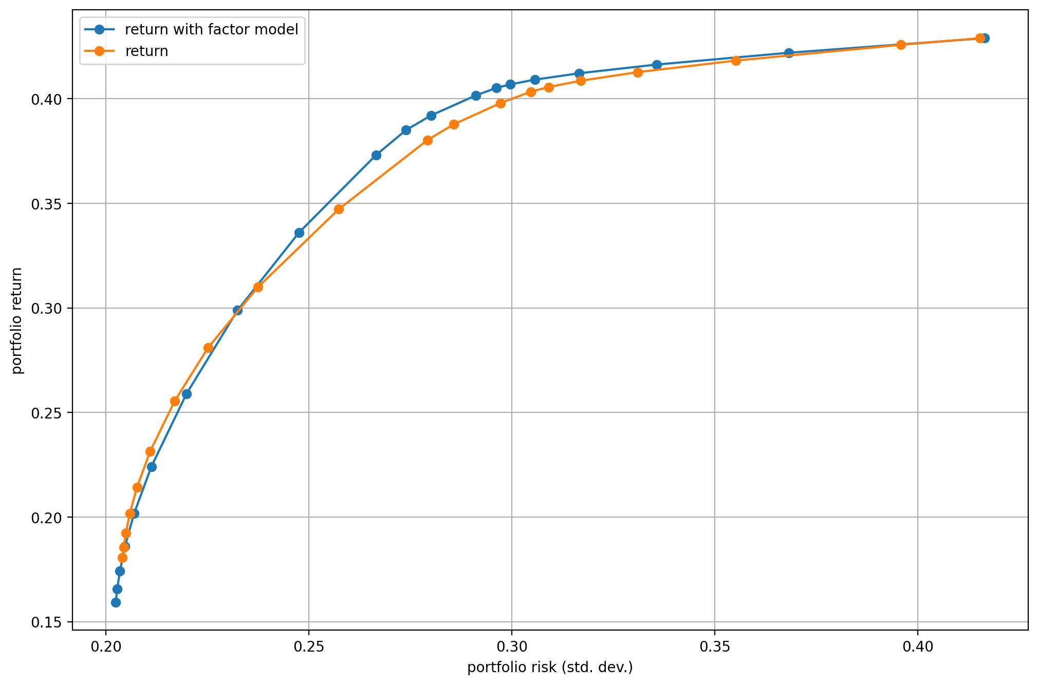
Fig. 5.1 The efficient frontier.

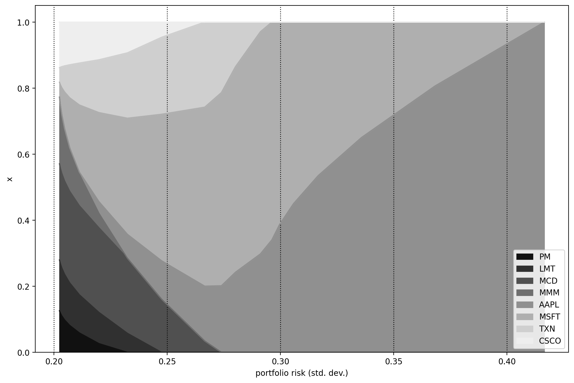
Fig. 5.2 Portfolio composition \(\mathbf{x}\) with varying level if risk-aversion \(\delta\).

5.5.2 Large scale factor model

In this example we will generate Monte Carlo based return data and compare optimization runtime between the Cholesky decomposition based and factor model based representation of the covariance matrix.

The following function generates the data, and the factor model:

def random_factor_model(N, K, T):
    # Generate K uncorrelated, zero mean factors, with weighted variance
    S_F = np.diag(range(1, K + 1))
    rng = np.random.default_rng(seed=1)
    Z_F = rng.multivariate_normal(np.zeros(K), S_F, T).T

    # Generate random factor model parameters
    B = rng.normal(size=(N, K))
    a = rng.normal(loc=1, size=(N, 1))
    e = rng.multivariate_normal(np.zeros(N), np.eye(N), T).T

    # Generate N time-series from the factors
    Z = a + B @ Z_F + e

    # Residual covariance
    S_theta = np.cov(e)
    diag_S_theta = np.diag(S_theta)

    # Optimization parameters
    m = np.mean(Z, axis=1)
    S = np.cov(Z)

    return m, S, B, S_F, diag_S_theta

The following code computes the comparison by increasing the number of securities \(N\). The factor model in this example will have \(K=10\) common factors, which is kept constant, because it typically does not depend on \(N\).

# Risk limit
gamma2 = 0.1

# Number of factors
K = 10

# Generate runtime data
list_runtimes_orig = []
list_runtimes_factor = []
for n in range(5, 15):
    N = 2**n
    T = N + 2**(n-1)
    m, S, B, S_F, diag_S_theta = random_factor_model(N, K, T)

    F = np.linalg.cholesky(S_F)
    G_factor = B @ F
    g_specific = np.sqrt(diag_S_theta)

    G_orig = np.linalg.cholesky(S)

    optimum_orig, runtime_orig = Markowitz(N, m, G_orig, gamma2)
    optimum_factor, runtime_factor = Markowitz(N, m, (G_factor, g_specific), gamma2)
    list_runtimes_orig.append((N, runtime_orig))
    list_runtimes_factor.append((N, runtime_factor))

tup_N_orig, tup_time_orig = list(zip(*list_runtimes_orig))
tup_N_factor, tup_time_factor = list(zip(*list_runtimes_factor))

The function call Markowitz(N, m, G, gamma2) runs the Fusion model, the same way as in Sec. 2.4 (Example). If instead of the argument G we specify the tuple (G_factor, g_specific), then the risk constraint in the Fusion model is created such that it exploits the risk factor structure:

# M is the Fusion model object
factor_risk = Expr.mul(G_factor.T, x)
specific_risk = Expr.mulElm(g_specific, x)
total_risk = Expr.vstack(factor_risk, specific_risk)

M.constraint('risk', Expr.vstack(np.sqrt(gamma2), total_risk), Domain.inQCone())

To get the runtime of the optimization, we add the following line to the model:

time = M.getSolverDoubleInfo("optimizerTime")

The results can be seen on Fig. 5.3, showing that the factor model based covariance matrix modeling can result in orders of magnitude faster solution times for large scale problems.

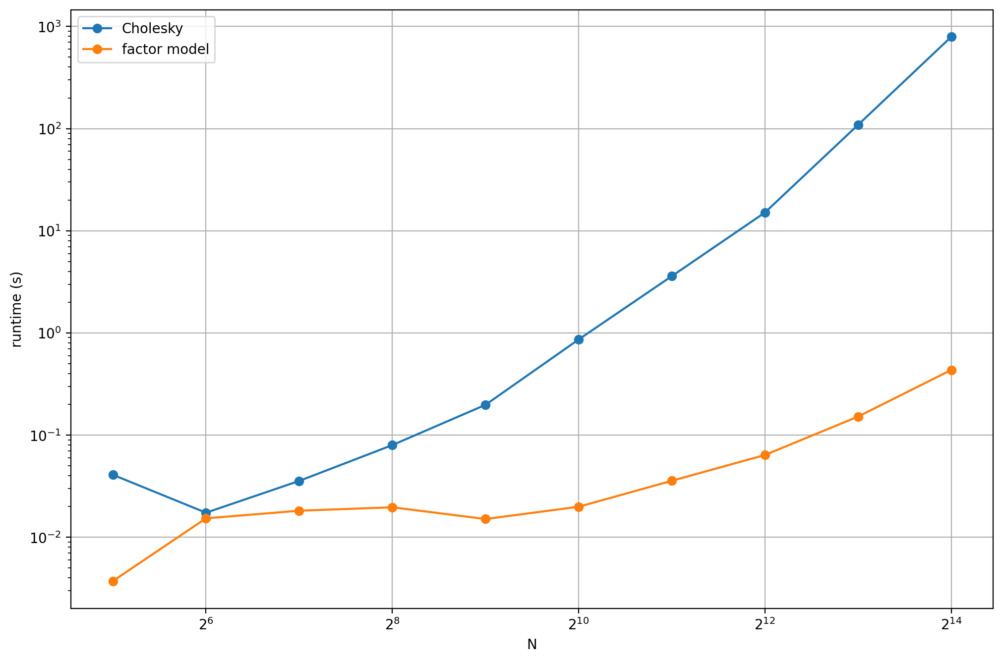
Fig. 5.3 Runtimes with and without using a factor model.

Footnotes

[1]

For a white noise process \(\varepsilon_t\) we have \(\mathbb{E}(\varepsilon_t) = \mathbf{0}\) and \(\mathrm{Cov}(\varepsilon_{t_1}, \varepsilon_{t_2}) = \Omega\) if \(t_1 = t_2\), where \(\Omega\) does not depend on \(t\), otherwise \(\mathbf{0}\).

[2]

If \(\Sigma_\varepsilon\) is not diagonal then we have an approximate factor model.

[3]

Additional lags of \(F_t\) in the \(Z_t\) equations can be easily allowed, then we obtain a dynamic factor model.

[4]

This is because \(\mathbf{c}\mathbf{c}^\mathsf{T}\circ(\EBeta\ECov_F\EBeta^\mathsf{T}+\ECov_\theta) = [\mathrm{Diag}(\mathbf{c})\EBeta]\ECov_F[\mathrm{Diag}(\mathbf{c})\EBeta]^\mathsf{T}+\mathrm{Diag}(\mathbf{c}\circ\mathbf{c})\ECov_\theta\).