2 Markowitz portfolio optimization

In this section we introduce the Markowitz model in portfolio optimization, and discuss its different formulations and the most important input parameters.

2.1 The mean–variance model

Consider an investor who wishes to allocate capital among $N$ securities at time $t=0$ and hold them over a single period of time until $t=h$. We denote $p_{0,i}$ the (known) price of security $i$ at the beginning of the investment period and $P_{h,i}$ the (random) price of security $i$ at the end of the investment period $t=h$. The rate of return of security $i$ over period $h$ is then modeled by the random variable $R_i=P_{h,i}/p_{0,i}-1$, and its expected value is denoted by ${\mu }_i=\mathbb{E}(R_i)$. The risk-averse investor seeks to maximize the return of the investment, while trying to keep the investment risk, i. e., the uncertainty of the future security returns $R_i$ on an acceptable low level.

The part of investment risk called specific risk (the risk associated with each individual security) can be reduced (for a fixed expected rate of return) through diversification, which means the selection of multiple unrelated securities into a portfolio. [1] Modern Portfolio Theory formalized this process by using variance as a measure of portfolio risk, and constructing a optimization problem.

Thus we make the investment decision at time $t=0$ by specifying the $N$-dimensional decision vector $\mathbf{x}$ called portfolio, where $x_i$ is the fraction of funds invested into security $i$. We can then express the random portfolio return as $R_{\mathbf{x}}=\sum _i{x}_i{R}_i={\mathbf{x}}^{\mathsf{T}}R$, where $R$ is the vector of security returns. The optimal $\mathbf{x}$ is given based on the following inputs of the portfolio optimization problem:

• The expected portfolio return

  $${\mu }_{\mathbf{x}}=\mathbb{E}(R_{\mathbf{x}})={\mathbf{x}}^{\mathsf{T}}\mathbb{E}(R)={\mathbf{x}}^{\mathsf{T}}\mu .$$

• The portfolio variance

  $${\sigma }_{\mathbf{x}}^2=\mathrm{Var}(R_{\mathbf{x}})=\sum _i\mathrm{Cov}(R_i,R_j)x_i{x}_j={\mathbf{x}}^{\mathsf{T}}\mathrm{\Sigma }\mathbf{x}.$$

Here $\mu$ is the vector of expected returns, $\mathrm{\Sigma }$ is the covariance matrix of returns, summarizing the risks associated with the securities. Note that the covariance matrix is symmetric positive semidefinite by definition, and if we assume that none of the securities is redundant [2], then it is positive definite. This can also be seen if we consider that the portfolio variance must always be a positive number. After the above parameters the problem is also referred to as mean–variance optimization (MVO). The choice of variance as the risk measure results that MVO is a quadratic optimization (QO) problem. [3]

Using these input parameters, the MVO problem seeks to select a portfolio of securities $\mathbf{x}$ in such a way that it finds the optimal tradeoff between expected portfolio return and portfolio risk. In other words it seeks to maximize the return while limiting the level of risk, or it wants to minimize the risk while demanding at least a given level of return. Thus portfolio optimization can be seen as a bi-criteria optimization problem.

2.1.1 Solution of the mean–variance model

To be able to solve the portfolio optimization problem, we have to assume that the investor knows the value of the expected return vector $\mu$ and covariance matrix $\mathrm{\Sigma }$. In practice it is only possible to have estimates, which we will denote by $\mathit{\mu }$ and $\mathbf{\Sigma }$ respectively. (Details on the properties of these estimates and ways to improve them will be the topic of Sec. 4 (Dealing with estimation error).)

In the simplest form of the MVO problem only risky securities are considered. Also the portfolio is fully invested with no initial holdings, implying the linear equality constraint $\sum _i{x}_i={\mathbf{1}}^{\mathsf{T}}\mathbf{x}=1$, where $\mathbf{1}$ denotes a vector of ones.

We can formulate this portfolio optimization problem in three equivalent ways:

1. Minimize the portfolio risk, with the constraint expressing a lower bound on the portfolio return:

   (2.1)$$\begin{array}{r}\begin{array}{lrcl}\text{minimize}& {\mathbf{x}}^{\mathsf{T}}\mathbf{\Sigma }\mathbf{x}& & \\ \text{subject to}& {\mathit{\mu }}^{\mathsf{T}}\mathbf{x}& \ge & r_{\min },\\ & {\mathbf{1}}^{\mathsf{T}}\mathbf{x}& =& 1.\end{array}\end{array}$$

   Here $r_{\min }$ is the target expected return, which the investor wishes to reach. In this problem the objective function is convex quadratic, all the constraints are linear, thus it is a quadratic optimization (QO) problem. While QO problems are easy to solve, this formulation is not ideal in practice because investors might prefer specifying an upper bound on the portfolio risk instead of specifying a lower bound on the expected portfolio return.

2. Maximize the expected portfolio return, with the constraint expressing an upper bound on the portfolio risk:

   (2.2)$$\begin{array}{r}\begin{array}{lrcl}\text{maximize}& {\mathit{\mu }}^{\mathsf{T}}\mathbf{x}& & \\ \text{subject to}& {\mathbf{x}}^{\mathsf{T}}\mathbf{\Sigma }\mathbf{x}& \le & {\gamma }^2,\\ & {\mathbf{1}}^{\mathsf{T}}\mathbf{x}& =& 1.\end{array}\end{array}$$

   In this formulation it is possible to explicitly constrain the risk measure (the variance), which makes it more practical. We can also add constraints on multiple types of risk measures more easily. However, the problem in this form is not a QO because of the quadratic constraint. We can reformulate it as a conic problem; see Sec. 2.3 (Conic formulation).

3. Maximize the utility function of the investor:

   (2.3)$$\begin{array}{r}\begin{array}{lrcl}\text{maximize}& {\mathit{\mu }}^{\mathsf{T}}\mathbf{x}-\frac{\delta }{2}{\mathbf{x}}^{\mathsf{T}}\mathbf{\Sigma }\mathbf{x}& & \\ \text{subject to}& {\mathbf{1}}^{\mathsf{T}}\mathbf{x}& =& 1.\end{array}\end{array}$$

   In this case we construct the (concave) quadratic utility function ${\mathit{\mu }}^{\mathsf{T}}\mathbf{x}-\frac{\delta }{2}{\mathbf{x}}^{\mathsf{T}}\mathbf{\Sigma }\mathbf{x}$ to represent the risk-averse investor’s preferred tradeoff between portfolio return and portfolio risk. This preference can be adjusted using the risk-aversion coefficient $\delta$. However this parameter might not have intuitive investment meaning for the investor.

   We get a variant of this optimization problem by using the standard deviation instead of the variance:

   (2.4)$$\begin{array}{r}\begin{array}{lrcl}\text{maximize}& {\mathit{\mu }}^{\mathsf{T}}\mathbf{x}-\tilde{\delta }\sqrt{{\mathbf{x}}^{\mathsf{T}}\mathbf{\Sigma }\mathbf{x}}& & \\ \text{subject to}& {\mathbf{1}}^{\mathsf{T}}\mathbf{x}& =& 1.\end{array}\end{array}$$

   This form is favorable because then the standard deviation penalty term will be of the same scale as portfolio return.

   Moreover, if we assume portfolio return to be normally distributed, then $\tilde{\delta }$ has a more tangible meaning; it is the z-score [4] of portfolio return. Also, the objective function will be the $(1-\alpha )$-quantile of portfolio return, which is the opposite of the $\alpha$ confidence level value-at-risk (VaR). The number $\alpha$ comes from $\mathrm{\Phi }(-\tilde{\delta })=1-\alpha$, where $\mathrm{\Phi }$ is the cumulative distribution function of the normal distribution.

   We can see that for $\tilde{\delta }=0$ we maximize expected portfolio return. Then by increasing $\tilde{\delta }$ we put more and more weight on tail risk, i. e., we maximize a lower and lower quantile of portfolio return. This makes selection of $\tilde{\delta }$ more intuitive in practice. Note that computing quantiles is more complicated for other distributions, because in general they are not determined by only mean and standard deviation.

   These two problems will result in the same set of optimal solutions as the other two formulations. They also allow an easy computation of the entire efficient frontier. Maximizing problem (2.3) is again a QO, but problem (2.4) is not because of the square root. This latter problem can be solved using conic reformulation, as we will see in Sec. 2.3 (Conic formulation).

The optimal portfolio $\mathbf{x}$ computed by the Markowitz model is efficient in the sense that there is no other portfolio giving a strictly higher return for the same amount of risk or a strictly lower risk for the same amount of return. In other words an efficient portfolio is Pareto optimal. The collection of such points form the efficient frontier in mean return–variance space.

The above introduced simple formulations are trivial to solve. Through the method of Lagrangian multipliers we can get analytical formulas, which involve $\mathit{\mu }$ and ${\mathbf{\Sigma }}^{-1}$ as parameters. Thus the solution is simply to invert the covariance matrix (see e. g. in [CJPT18]). This makes them useful as a demonstration example, but they have only limited investment value.

2.2 Constraints, modifications

In investment practice additional constraints are essential, and it is common to add linear equalities and inequalities, convex inequalities, and/or extra objective function terms to the model, which represent various restrictions on the optimal security weights.

Constraints can reflect investment strategy or market outlook information, they can be useful for imposing quality controls on the portfolio management process, or for controlling portfolio structure and avoiding inadvertent risk exposures. In these more realistic use cases however, only numerical optimization algorithms are suitable for finding the solution.

In the following, we discuss some of the constraints commonly added to portfolio optimization problems.

2.2.1 Budget constraint

In general we can assume that we have ${\mathbf{x}}_0$ fraction of initial holdings, and $x_0^{\mathrm{f}}$ fraction of (risk-free) initial wealth to invest into risky securities. Then ${\mathbf{1}}^{\mathsf{T}}{\mathbf{x}}_0+x_0^{\mathrm{f}}=1$ is an initial condition, meaning that both the risky and the risk-free securities take up some fraction of the initial portfolio. After portfolio optimization, the portfolio composition changes, but no cash is added to or taken out from the portfolio. Thus the condition

(2.5)$${\mathbf{1}}^{\mathsf{T}}\mathbf{x}+x^{\mathrm{f}}=1$$

has to hold. For the differences $\tilde{\mathbf{x}}=\mathbf{x}-{\mathbf{x}}_0$ and ${\tilde{x}}^{\mathrm{f}}=x^{\mathrm{f}}-x_0^{\mathrm{f}}$ it follows that ${\mathbf{1}}^{\mathsf{T}}\tilde{\mathbf{x}}+{\tilde{x}}^{\mathrm{f}}=0$ has to hold.

If we do not want to keep any wealth in the risk-free security, then in addition $x^{\mathrm{f}}$ must be zero.

2.2.2 Diversification constraints

These constraints can help limit portfolio risk by limiting the exposure to individual positions or industries, sectors.

For a single position, they can be given in the form

$$l_i\le x_i\le u_i.$$

For a group of securities such as an industry or sector, represented by the set $\mathcal{I}$ they will be

$$l_i\le \sum _{i\in \mathcal{I}}{x}_i\le u_i.$$

We can also create a constraint that limits the total fraction of the $m$ largest investments to at most $p$. Based on Sec. 13.1.1.4 (Sum of largest elements) this is represented by the following set of constraints:

$$mt+{\mathbf{1}}^T\mathbf{u}\le p,\mathbf{u}+t\ge \mathbf{x},\mathbf{u}\ge 0,$$

where $\mathbf{u}$ and $t$ are new variables.

2.2.3 Leverage constraints

2.2.3.1 Componentwise short sale limit

The simplest form of leverage constraint is when we do not allow any short selling. This is the long-only constraint stated as

$$\mathbf{x}\ge 0.$$

We can allow some amount of short selling $s_i$ on security $i$ by stating

$$x_i\ge -s_i.$$

2.2.3.2 Total short sale limit

We can also bound the total short selling by the constraint

$$\sum _i\max (-x_i,0)\le S.$$

We can rewrite this as a set of linear constraints by modeling the maximum function based on Sec. 13.1.1.1 (Maximum function) using an auxiliary vector ${\mathbf{t}}^{-}$:

$${\mathbf{1}}^{\mathsf{T}}{\mathbf{t}}^{-}\le S,{\mathbf{t}}^{-}\ge -\mathbf{x},{\mathbf{t}}^{-}\ge 0.$$

2.2.3.3 Collateralization requirement

An interesting variant of this constraint is the collateralization requirement, which limits the total of short positions to a fraction of the total of long positions. We can model it by introducing new variables ${\mathbf{x}}^{+}$ and ${\mathbf{x}}^{-}$ for the long and short part of $\mathbf{x}$, based on Sec. 13.1.1.2 (Positive and negative part). Then the collateralization requirement will be:

$$\sum _i{x}_i^{-}\le c\sum _i{x}_i^{+}.$$

2.2.3.4 Leverage strategy

A leverage strategy is to do short selling, then use the proceeds to buy other securities. We can express such a strategy in general using two constraints:

• ${\mathbf{1}}^{\mathsf{T}}\mathbf{x}=1$,

• $\sum _i|x_i|\le c$ or equivalently $\Vert \mathbf{x}{\Vert }_1\le c$,

where $c=1$ yields the long-only constraint and $c=1.6$ means the 130/30 strategy. The 1-norm constraint is nonlinear, but can be modeled as a linear constraint based on Sec. 13.1.1.6 (Manhattan norm (1-norm)): $-\mathbf{z}\le \mathbf{x}\le \mathbf{z},{\mathbf{1}}^{\mathsf{T}}\mathbf{z}=c$.

2.2.4 Turnover constraints

The turnover constraint limits the total change in the portfolio positions, which can help limiting e. g. taxes and cost of transactions.

Suppose ${\mathbf{x}}_0$ is the initial holdings vector. Then we can write the turnover constraint as

$$\Vert \mathbf{x}-{\mathbf{x}}_0{\Vert }_1\le c.$$

This nonlinear expression can be modeled as linear constraint using Sec. 13.1.1.6 (Manhattan norm (1-norm)).

2.2.5 Practical considerations

We can of course add many other constraints that might be imposed by regulations or arise from specific investor preferences. As long as all of these are linear or conic, the problem will not become significantly harder to solve. (See Sec. 13.1 (Conic optimization refresher) for a summary on conic constraints.)

However, we must not add too many constraints. Overconstraining a portfolio can lead to infeasibility of the optimization problem, or even if there exists a solution, out-of-sample performance of it could be poor.

Throughout this book the general notation $\mathbf{x}\in \mathcal{F}$ will indicate any further constraints added to the problem, that are not relevant to the given example. Then we can write the general MVO problem in the form

(2.6)$$\begin{array}{r}\begin{array}{lrcl}\text{maximize}& {\mathit{\mu }}^{\mathsf{T}}\mathbf{x}& & \\ \text{subject to}& {\mathbf{x}}^{\mathsf{T}}\mathbf{\Sigma }\mathbf{x}& \le & {\gamma }^2,\\ & \mathbf{x}& \in & \mathcal{F}.\end{array}\end{array}$$

2.3 Conic formulation

We have seen that some of the portfolio optimization problems in Sec. 2.1.1 (Solution of the mean–variance model) are quadratic optimization problems. Solving QO problems in their original form is popular and considered easy, because this model was studied starting from early in history (in the 1950s), allowing it to become a well known and mature approach. However, more recent results show us that conic optimization models can improve on QO models both in the theoretical and in the practical sense. More on this in Sec. 13.1.2 (Traditional quadratic models).

In this section we will show to convert problems (2.1)-(2.4) into conic form. Assuming that the covariance matrix estimate $\mathbf{\Sigma }$ is positive definite, it is possible to decompose it as $\mathbf{\Sigma }=\mathbf{G}{\mathbf{G}}^{\mathsf{T}}$, where $\mathbf{G}\in {\mathbb{R}}^{N\times k}$. We can do this for example by Cholesky decomposition, see Sec. 13.1.1.10 (Quadratic form) for a list of other possibilities. An interesting approach in financial applications is the factor model, which can have the advantage of having a direct financial interpretation (see in Sec. 5 (Factor models)).

Even if there are no redundant securities, $\mathbf{\Sigma }$ can be positive semidefinite if the number of samples is lower than the number of securities. In this case the Cholesky decomposition might not be computable. [5] We can then apply regularization techniques (e. g. shrinkage, see in Sec. 4.2.1 (Covariance shrinkage)) to ensure positive definiteness. Otherwise if suitable linear returns data (see in Sec. 3 (Input data preparation)) is available, then a centered and normalized data matrix can also serve as matrix $\mathbf{G}$.

Using the decomposition we can write the portfolio variance as ${\mathbf{x}}^{\mathsf{T}}\mathbf{\Sigma }\mathbf{x}={\mathbf{x}}^{\mathsf{T}}\mathbf{G}{\mathbf{G}}^{\mathsf{T}}\mathbf{x}=\Vert {\mathbf{G}}^{\mathsf{T}}\mathbf{x}{\Vert }_2^2$. This leads to two different conic forms (see also in Sec. 13.1.1.10 (Quadratic form)).

1. Modeling with rotated quadratic cone:

   We can directly model the squared norm constraint $\Vert {\mathbf{G}}^{\mathsf{T}}\mathbf{x}{\Vert }_2^2\le {\gamma }^2$ using the rotated quadratic cone as $({\gamma }^2,\frac{1}{2},{\mathbf{G}}^{\mathsf{T}}\mathbf{x})\in {\mathcal{Q}}_{\mathrm{r}}^{k+2}$. This will give us the conic equivalent of e. g. problem (2.3):

   (2.7)$$\begin{array}{r}\begin{array}{lrcl}\text{maximize}& {\mathit{\mu }}^{\mathsf{T}}\mathbf{x}& & \\ \text{subject to}& ({\gamma }^2,\frac{1}{2},{\mathbf{G}}^{\mathsf{T}}\mathbf{x})& \in & {\mathcal{Q}}_{\mathrm{r}}^{k+2},\\ & {\mathbf{1}}^{\mathsf{T}}\mathbf{x}& =& 1.\end{array}\end{array}$$

2. Modeling with quadratic cone:

   We can also consider the equivalent norm constraint $\Vert {\mathbf{G}}^{\mathsf{T}}\mathbf{x}{\Vert }_2\le \gamma$ instead of the squared norm, and model it using the quadratic cone as $(\gamma ,{\mathbf{G}}^{\mathsf{T}}\mathbf{x})\in {\mathcal{Q}}^{k+1}$. The conic equivalent of problem (2.3) will then look like

   (2.8)$$\begin{array}{r}\begin{array}{lrcl}\text{maximize}& {\mathit{\mu }}^{\mathsf{T}}\mathbf{x}& & \\ \text{subject to}& (\gamma ,{\mathbf{G}}^{\mathsf{T}}\mathbf{x})& \in & {\mathcal{Q}}^{k+1},\\ & {\mathbf{1}}^{\mathsf{T}}\mathbf{x}& =& 1.\end{array}\end{array}$$

   This way we can also model problem (2.4). We introduce the variable $s$ to represent the upper bound of the portfolio standard deviation, and model the constraint $\Vert {\mathbf{G}}^{\mathsf{T}}\mathbf{x}{\Vert }_2\le s$ using the quadratic cone as

   (2.9)$$\begin{array}{r}\begin{array}{lrcl}\text{maximize}& {\mathit{\mu }}^{\mathsf{T}}\mathbf{x}-\tilde{\delta }s& & \\ \text{subject to}& (s,{\mathbf{G}}^{\mathsf{T}}\mathbf{x})& \in & {\mathcal{Q}}^{k+1},\\ & {\mathbf{1}}^{\mathsf{T}}\mathbf{x}& =& 1.\end{array}\end{array}$$

   While modeling problem (2.3) using the rotated quadratic cone might seem more natural, it can also be reasonable to model it using the quadratic cone for the benefits of the smaller scale and intuitive interpretation of $\tilde{\delta }$. This is the same as modeling of problem (2.4), which shows that conic optimization can also provide efficient solution to problems that are inefficient to solve in their original form.

In general, transforming the optimization problem into the conic form has multiple practical advantages. Solving the problem in this format will result in a more robust and usually faster and more reliable solution process. Check Sec. 13.1.2 (Traditional quadratic models) for details.

2.4 Example

We have seen how to transform a portfolio optimization problem into conic form. Now we will present a detailed example in MOSEK Fusion. Assume that the input data estimates $\mathit{\mu }$ and $\mathbf{\Sigma }$ are given. The latter is also positive definite. For methods and examples on how to obtain these see Sec. 3 (Input data preparation).

Suppose we would like to create a long only portfolio of eight stocks. Assume that we receive the following variables:

# Expected returns and covariance matrix
m = np.array(
    [0.0720, 0.1552, 0.1754, 0.0898, 0.4290, 0.3929, 0.3217, 0.1838]
)
S = np.array([
    [0.0946, 0.0374, 0.0349, 0.0348, 0.0542, 0.0368, 0.0321, 0.0327],
    [0.0374, 0.0775, 0.0387, 0.0367, 0.0382, 0.0363, 0.0356, 0.0342],
    [0.0349, 0.0387, 0.0624, 0.0336, 0.0395, 0.0369, 0.0338, 0.0243],
    [0.0348, 0.0367, 0.0336, 0.0682, 0.0402, 0.0335, 0.0436, 0.0371],
    [0.0542, 0.0382, 0.0395, 0.0402, 0.1724, 0.0789, 0.0700, 0.0501],
    [0.0368, 0.0363, 0.0369, 0.0335, 0.0789, 0.0909, 0.0536, 0.0449],
    [0.0321, 0.0356, 0.0338, 0.0436, 0.0700, 0.0536, 0.0965, 0.0442],
    [0.0327, 0.0342, 0.0243, 0.0371, 0.0501, 0.0449, 0.0442, 0.0816]
])

The similar magnitude and positivity of all the covariances suggests that the selected securities are closely related. In Sec. 3.4.2 (Data collection) we will see that they are indeed from the same market and that the data was collected from a highly bullish time period, resulting in the large expected returns. Later in Sec. 5.5.1 (Single factor model) we will analyze this covariance matrix more thoroughly.

2.4.1 Maximizing return

We will solve problem (2.2) with an additional constraint to prevent short selling. We specify a risk level of ${\gamma }^2=0.05$ and assume that there are no transaction costs. The optimization problem will then be

(2.10)$$\begin{array}{r}\begin{array}{lrcl}\text{maximize}& {\mathit{\mu }}^{\mathsf{T}}\mathbf{x}& & \\ \text{subject to}& {\mathbf{x}}^{\mathsf{T}}\mathbf{\Sigma }\mathbf{x}& \le & {\gamma }^2,\\ & {\mathbf{1}}^{\mathsf{T}}\mathbf{x}& =& 1,\\ & \mathbf{x}& \ge & 0.\end{array}\end{array}$$

Recall that by the Cholesky decomposition we have $\mathbf{\Sigma }=\mathbf{G}{\mathbf{G}}^{\mathsf{T}}$. Then we can model the quadratic term ${\mathbf{x}}^{\mathsf{T}}\mathbf{\Sigma }\mathbf{x}\le {\gamma }^2$ using the rotated quadratic cone as $({\gamma }^2,\frac{1}{2},{\mathbf{G}}^{\mathsf{T}}\mathbf{x})\in {\mathcal{Q}}_{\mathrm{r}}^{N+2}$, and arrive at

(2.11)$$\begin{array}{r}\begin{array}{lrcl}\text{maximize}& {\mathit{\mu }}^{\mathsf{T}}\mathbf{x}& & \\ \text{subject to}& ({\gamma }^2,\frac{1}{2},{\mathbf{G}}^{\mathsf{T}}\mathbf{x})& \in & {\mathcal{Q}}_{\mathrm{r}}^{N+2},\\ & {\mathbf{1}}^{\mathsf{T}}\mathbf{x}& =& 1,\\ & \mathbf{x}& \ge & 0.\end{array}\end{array}$$

In the code, $\mathbf{G}$ will be an input parameter, so we compute it first. We use the Python package numpy for this purpose, abbreviated here as np.

N = m.shape[0]  # Number of securities
gamma2 = 0.05  # Risk limit

# Cholesky factor of S to use in conic risk constraint
G = np.linalg.cholesky(S)

Next we define the Fusion model for problem (2.11):

with Model("MarkowitzReturn") as M:
     # Decision variable (fraction of holdings in each security)
     # The variable x is the fraction of holdings in each security.
     # x must be positive, this imposes the no short-selling constraint.
     x = M.variable("x", N, Domain.greaterThan(0.0))

     # Budget constraint
     M.constraint('budget', Expr.sum(x) == 1)

     # Objective
     M.objective('obj', ObjectiveSense.Maximize, x.T @ m)

     # Imposes a bound on the risk
     M.constraint('risk', Expr.vstack(gamma2, 0.5, G.T @ x),
                          Domain.inRotatedQCone())

     # Solve optimization
     M.solve()

     returns = M.primalObjValue()
     portfolio = x.level()

The resulting portfolio return is ${\mathit{\mu }}^{\mathsf{T}}\mathbf{x}=0.2767$ and the portfolio composition is $\mathbf{x}=[0,0.0913,0.2691,0,0.0253,0.3216,0.1765,0.1162]$.

2.4.2 Efficient frontier

In this section we compute the full efficient frontier using the same input variables. This is the easiest to do based on the formulation (2.3) by varying the delta parameter. We also prevent short selling in this case and assume no transaction costs. The optimization problem becomes

(2.12)$$\begin{array}{r}\begin{array}{lrcl}\text{maximize}& {\mathit{\mu }}^{\mathsf{T}}\mathbf{x}-\tilde{\delta }\sqrt{{\mathbf{x}}^{\mathsf{T}}\mathbf{\Sigma }\mathbf{x}}& & \\ \text{subject to}& {\mathbf{1}}^{\mathsf{T}}\mathbf{x}& =& 1,\\ & \mathbf{x}& \ge & 0.\end{array}\end{array}$$

With the help of Cholesky decomposition, we can model the quadratic term $\sqrt{{\mathbf{x}}^{\mathsf{T}}\mathbf{\Sigma }\mathbf{x}}=\sqrt{{\mathbf{x}}^{\mathsf{T}}\mathbf{G}{\mathbf{G}}^{\mathsf{T}}\mathbf{x}}=\Vert {\mathbf{G}}^{\mathsf{T}}\mathbf{x}{\Vert }_2$ in the objective as a conic constraint. Let us introduce the variable $s$ and apply that $\Vert {\mathbf{G}}^{\mathsf{T}}\mathbf{x}{\Vert }_2\le s$ is equivalent to the quadratic cone membership $(s,{\mathbf{G}}^{\mathsf{T}}\mathbf{x})\in {\mathcal{Q}}^{N+1}$. Then the problem will take the form

(2.13)$$\begin{array}{r}\begin{array}{lrcl}\text{maximize}& {\mathit{\mu }}^{\mathsf{T}}\mathbf{x}-\tilde{\delta }s& & \\ \text{subject to}& {\mathbf{1}}^{\mathsf{T}}\mathbf{x}& =& 1,\\ & \mathbf{x}& \ge & 0,\\ & (s,{\mathbf{G}}^{\mathsf{T}}\mathbf{x})& \in & {\mathcal{Q}}^{N+1}.\end{array}\end{array}$$

First we compute the input variable $\mathbf{G}$:

N = m.shape[0]  # Number of securities

# Cholesky factor of S to use in conic risk constraint
G = np.linalg.cholesky(S)

Next we define the Fusion model for problem (2.13):

with Model("MarkowitzFrontier") as M:
    # Variables
    # The variable x is the fraction of holdings in each security.
    # x must be positive, this imposes the no short-selling constraint.
    x = M.variable("x", N, Domain.greaterThan(0.0))

    # The variable s models the portfolio variance term in the objective.
    s = M.variable("s", 1, Domain.unbounded())

    # Budget constraint
    M.constraint('budget', Expr.sum(x) == 1)

    # Objective (quadratic utility version)
    delta = M.parameter()
    M.objective('obj', ObjectiveSense.Maximize,
                       x.T @ m - delta * s)

    # Conic constraint for the portfolio variance
    M.constraint('risk', Expr.vstack(s, G.T @ x), Domain.inQCone())

Here we use a feature in Fusion that allows us to define model parameters. The line delta = M.parameter() in the code does this. Defining a parameter is ideal for the computation of the efficient frontier, because it allows us to reuse an already existing optimization model, by only changing its parameter value.

To do so, we define the range of values for the risk aversion parameter $\delta$ to be $20$ numbers between ${10}^{-1}$ and ${10}^{1.5}$:

deltas = np.logspace(start=-1, stop=1.5, num=20)[::-1]

Then we will solve the optimization model repeatedly in a loop, setting a new value for the parameter $\delta$ in each iteration, without having to redefine the whole model each time.

columns = ["delta", "obj", "return", "risk"] + df_prices.columns.tolist()
df_result = pd.DataFrame(columns=columns)
for d in deltas:
    # Update parameter
    delta.setValue(d)

    # Solve optimization
    M.solve()

    # Save results
    portfolio_return = m @ x.level()
    portfolio_risk = s.level()[0]
    row = pd.Series([d, M.primalObjValue(), portfolio_return,
                     portfolio_risk] + list(x.level()), index=columns)
    df_result = df_result.append(row, ignore_index=True)

Then we can plot the results. See the risk-return plane on Fig. 2.1. We generate it by the following code:

# Efficient frontier
df_result.plot(x="risk", y="return", style="-o",
               xlabel="portfolio risk (std. dev.)",
               ylabel="portfolio return", grid=True)

We can observe the portfolio composition for different risk-aversion levels on Fig. 2.2, generated by

# Portfolio composition
my_cmap = LinearSegmentedColormap.from_list("non-extreme gray",
              ["#111111", "#eeeeee"], N=256, gamma=1.0)
df_result.set_index('risk').iloc[:, 3:].plot.area(colormap=my_cmap,
              xlabel='portfolio risk (std. dev.)', ylabel="x")

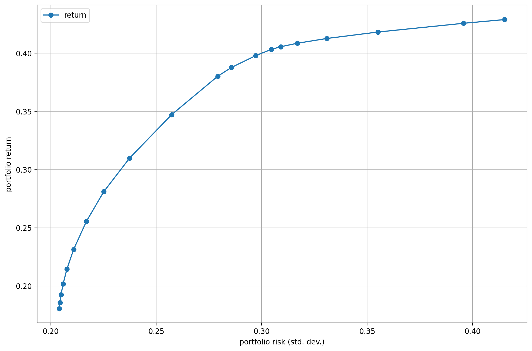
Fig. 2.1 The efficient frontier.

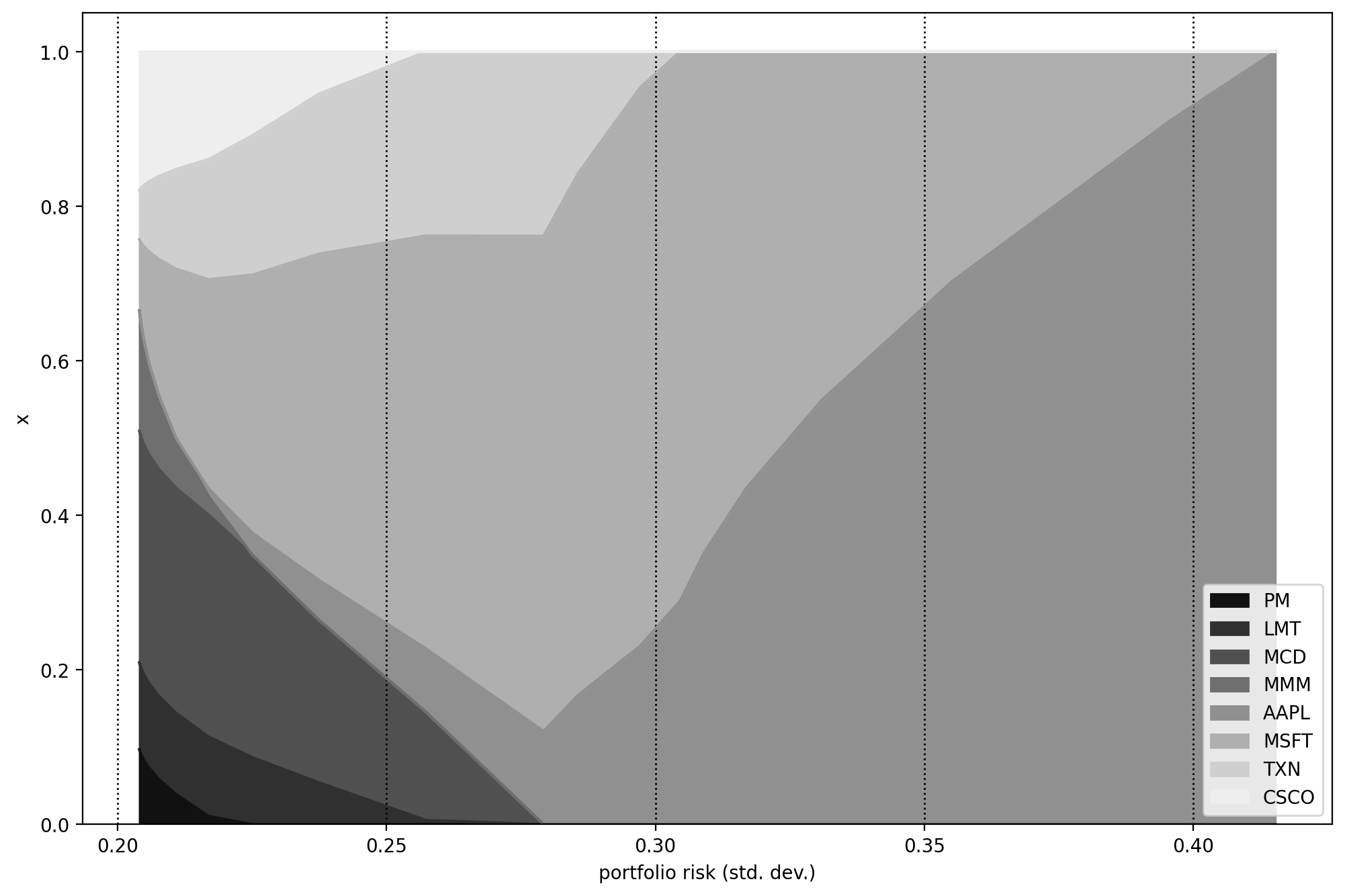
Fig. 2.2 Portfolio composition $\mathbf{x}$ with varying level if risk-aversion $\delta$.

Footnotes

[1]

The other component of risk called systematic risk can only be reduced by decreasing the expected return.

[2]

A security is redundant within the universe of securities in consideration, if there is a replicating portfolio, i. e., a combination of other securities in the universe, that has the same properties. It means that we can drop the redundant security from the universe without loss of opportunities for diversification. Keeping it in the portfolio could cause the covariance matrix $\mathrm{\Sigma }$ to be singular.

[3]

This was a reasonable choice from both the financial and the mathematical point of view, because modern portfolio theory and the theory of quadratic optimization started to develop about the same time in history, in the 1950s. However, the way we model risk can be different. See later in Sec. 8 (Other risk measures).

[4]

The z-score is the distance from the mean measured in units of standard deviation.

[5]

The Cholesky decomposition is possible for positive semidefinite matrices, but software implementations might need positive definiteness depending on the algorithm used (e. g. Python numpy).