10 Robust optimization

In chapter Sec. 4 (Dealing with estimation error) we have discussed in detail, that the inaccurate or uncertain input parameters of a portfolio optimization problem can result in wrong optimal solutions. In other words, the solution is very input sensitive. Robust optimization is another possible modeling tool to overcome this sensitivity. It is a way of handling estimation errors in the optimization problem instead of the input preparation phase. In the most common setup, the parameters are the estimated mean and estimated covariance matrix of the security returns. In robust optimization, we do not compute point estimates of these, but rather an uncertainty set, where the true values lie with certain confidence. A robust portfolio thus optimizes the worst-case performance with respect to all possible parameter values within their corresponding uncertainty sets. [CJPT18, VD09]

10.1 Types of uncertainty

We can form different types of uncertainty sets around the unknown parameters, depending on the nature of the uncertainty, the sensitivity of the solution, and the available information.

• Polytope: If we have a finite number of scenarios, we can form a polytope uncertainty set by taking the convex hull of the scenarios.

• Interval: We can compute a confidence interval for each of the parameters.

• Ellipsoidal region: For vector variables, we can compute confidence regions.

We can model all of these types of uncertainty sets in conic optimization, allowing us to solve robust optimization problems efficiently.

The size of the uncertainty sets reflects the desired level of robustness. For confidence intervals, it is controlled by the confidence level. There is of course a tradeoff, if the uncertainty sets are chosen to be very large, then the resulting portfolios will be very conservative, and they will perform much worse for any given parameter set, than the portfolio designed for that set of parameters. On the other hand, if the size is chosen too small, the resulting portfolio will not be robust enough.

10.2 Uncertainty in security returns

Consider problem (2.3), which we restate here:

(10.1)$$\begin{array}{r}\begin{array}{lrcl}\text{maximize}& {\mathit{\mu }}^{\mathsf{T}}\mathbf{x}-\frac{\delta }{2}{\mathbf{x}}^{\mathsf{T}}\mathbf{\Sigma }\mathbf{x}& & \\ \text{subject to}& {\mathbf{1}}^{\mathsf{T}}\mathbf{x}& =& 1.\end{array}\end{array}$$

Assume that the vector of mean returns $\mathit{\mu }$ belongs to the elliptical uncertainty set

(10.2)$${\mathcal{U}}_{\mu }=\{\mathit{\mu }\mid (\mathit{\mu }-{\mathit{\mu }}_0{)}^{\mathsf{T}}{Q}^{-1}(\mathit{\mu }-{\mathit{\mu }}_0)\le {\gamma }^2\},$$

where $Q$ is a known positive semidefinite matrix. Then the worst case expected portfolio return will be

$${\displaystyle \underset{\mathit{\mu }\in {\mathcal{U}}_{\mu }}{min}{\mathit{\mu }}^{\mathsf{T}}\mathbf{x}={\mathit{\mu }}_0^{\mathsf{T}}\mathbf{x}-\gamma \sqrt{{\mathbf{x}}^{\mathsf{T}}Q\mathbf{x}}.}$$

It follows that the robust version of (10.1) becomes

(10.3)$$\begin{array}{r}\begin{array}{lrcl}\text{maximize}& {\mathit{\mu }}_0^{\mathsf{T}}\mathbf{x}-\gamma \sqrt{{\mathbf{x}}^{\mathsf{T}}Q\mathbf{x}}-\frac{\delta }{2}{\mathbf{x}}^{\mathsf{T}}\mathbf{\Sigma }\mathbf{x}& & \\ \text{subject to}& {\mathbf{1}}^{\mathsf{T}}\mathbf{x}& =& 1.\end{array}\end{array}$$

10.3 Uncertainty in the factor model

In the article [GI03], the authors consider a factor model on security returns, treat its parameters as uncertain using ellipsoidal uncertainty sets defined as confidence regions, and formulate robust portfolio optimization problems.

Assume that for a random security return vector $R_t$ and factor return vector $F_t$ at time $t$, the factor model takes the form

(10.4)$$R_t=\mu +\beta F_t+{\theta }_t,$$

where $\mu$ is the vector of mean security returns, $\beta$ is the factor loading matrix, and ${\theta }_t$ is the vector of residual returns. We also assume an exact factor model (see Sec. 5 (Factor models)), meaning that the factor returns and residual returns are assumed to be independent, and the residual covariance matrix $D$ of ${\theta }_t$ is diagonal. Moreover, $\mathbb{E}(F_t)=\mathbf{0}$, so the factors carry no information on the mean returns. A final assumption in this section is that the factor covariance matrix $Q\in {\mathbb{R}}^{K\times K}$ is known exactly. This requirement will be relaxed later.

The portfolio mean return and portfolio variance will be $\mathbb{E}(R_{\mathbf{x}})={\mu }^{\mathsf{T}}\mathbf{x}$ and $\mathrm{Var}(R_{\mathbf{x}})={\mathbf{x}}^{\mathsf{T}}(\beta Q{\beta }^{\mathsf{T}}+D)\mathbf{x}$. If we compute estimates $\mathit{\mu }$, $\mathit{\beta }$, and $\mathbf{D}$ of the above quantities, we can reformulate problem (2.1):

(10.5)$$\begin{array}{r}\begin{array}{lrcl}\text{minimize}& t_1+t_2& & \\ \text{subject to}& {\mathit{\mu }}^{\mathsf{T}}\mathbf{x}& \ge & r_{\min },\\ & {\mathbf{x}}^{\mathsf{T}}\mathbf{D}\mathbf{x}& \le & t_2,\\ & {\mathbf{x}}^{\mathsf{T}}\mathit{\beta }Q{\mathit{\beta }}^{\mathsf{T}}\mathbf{x}& \le & t_1,\\ & \mathbf{x}& \in & \mathcal{F}.\end{array}\end{array}$$

10.3.1 Uncertainty sets

Instead of computing (10.5) using estimates, we assume variables $\mathit{\mu }$, $\mathit{\beta }$, and $\mathbf{D}$ to lie in the following uncertainty sets:

• The diagonal elements ${\sigma }_{\theta }^2$ of the matrix $\mathbf{D}$ can take values in an uncertainty interval $[{\underset{―}{\sigma }}_{\theta }^2,{\bar{\sigma }}_{\theta }^2]$:

  (10.6)$${\mathcal{U}}_D=\{\mathbf{D}\mid \mathrm{diag}(\mathbf{D})\in [{\underset{―}{\sigma }}_{\theta }^2,{\bar{\sigma }}_{\theta }^2]\}$$

• The factor loadings matrix $\mathit{\beta }$ belongs to the elliptical uncertainty set

  (10.7)$${\mathcal{U}}_{\beta }=\{\mathit{\beta }\mid \mathit{\beta }={\mathit{\beta }}_0+\mathbf{B},\Vert {\mathbf{B}}_i{\Vert }_{\mathbf{G}}\le {\rho }_i,i=1,\dots ,N\}$$

  where ${\mathbf{B}}_i$ is row $i$ of the matrix $\mathbf{B}$, and $\Vert \mathbf{b}{\Vert }_{\mathbf{G}}=\sqrt{{\mathbf{b}}^{\mathsf{T}}\mathbf{G}\mathbf{b}}$ denotes the elliptic norm of $\mathbf{b}$ with respect to the positive definite matrix $\mathbf{G}\in {\mathbb{R}}^{K\times K}$.

• The vector $\mathit{\mu }$ of mean returns is assumed to lie in the uncertainty interval

  (10.8)$${\mathcal{U}}_{\mu }=\{\mathit{\mu }\mid \mathit{\mu }={\mathit{\mu }}_0+\mathbf{m},|\mathbf{m}|\le \gamma \}$$

10.3.2 Robust problem formulation

The goal of robust portfolio selection is then to select portfolios that perform well for all parameter values that constitute these sets of uncertainty. In other words, we are looking for worst case optimal solutions, formulated as minmax optimization problems. Then we can state the robust mean-variance optimization problem:

(10.9)$$\begin{array}{r}\begin{array}{lrcl}\text{minimize}& t_1+t_2& & \\ \text{subject to}& {\displaystyle \underset{\mathit{\mu }\in {\mathcal{U}}_{\mu }}{min}{\mathit{\mu }}^{\mathsf{T}}\mathbf{x}}& \ge & r_{\min },\\ & {\displaystyle \underset{\mathbf{D}\in {\mathcal{U}}_D}{max}{\mathbf{x}}^{\mathsf{T}}\mathbf{D}\mathbf{x}}& \le & t_2,\\ & {\displaystyle \underset{\mathit{\beta }\in {\mathcal{U}}_{\beta }}{max}{\mathbf{x}}^{\mathsf{T}}\mathit{\beta }Q{\mathit{\beta }}^{\mathsf{T}}\mathbf{x}}& \le & t_1,\\ & \mathbf{x}& \in & \mathcal{F}.\end{array}\end{array}$$

To convert the minmax problem (10.9) into a conic optimization problem, we first need to represent the worst case expected portfolio return and portfolio variance using conic constraints:

• We can evaluate the worst case expected portfolio return:

  $${\displaystyle \underset{\mathit{\mu }\in {\mathcal{U}}_{\mu }}{min}{\mathit{\mu }}^{\mathsf{T}}\mathbf{x}={\mathit{\mu }}_0^{\mathsf{T}}\mathbf{x}-{\gamma }^{\mathsf{T}}|\mathbf{x}|.}$$

• We can evaluate the worst case residual portfolio variance:

  $${\displaystyle \underset{\mathbf{D}\in {\mathcal{U}}_D}{max}{\mathbf{x}}^{\mathsf{T}}\mathbf{D}\mathbf{x}={\mathbf{x}}^{\mathsf{T}}\mathrm{Diag}({\bar{\sigma }}_{\theta }^2)\mathbf{x}.}$$

• We cannot easily evaluate the worst case factor portfolio variance. But we can show that the constraint

  $$\underset{\mathit{\beta }\in {\mathcal{U}}_{\beta }}{max}{\mathbf{x}}^{\mathsf{T}}\mathit{\beta }Q{\mathit{\beta }}^{\mathsf{T}}\mathbf{x}\le t_1$$

  is equivalent to

  (10.10)$$({\rho }^{\mathsf{T}}|\mathbf{x}|,t_1,\mathbf{x})\in \mathcal{H}({\mathit{\beta }}_0,Q,\mathbf{G}).$$

  Relation (10.10) is a shorthand notation for the following: Define $\mathbf{H}={\mathbf{G}}^{-1/2}Q{\mathbf{G}}^{-1/2}$, with spectral decomposition $\mathbf{H}=\mathbf{V}\mathrm{\Lambda }{\mathbf{V}}^{\mathsf{T}}$, and define $\mathbf{w}={\mathbf{V}}^{\mathsf{T}}{\mathbf{H}}^{1/2}{\mathbf{G}}^{1/2}{\mathit{\beta }}_0^{\mathsf{T}}\mathbf{x}$. Then there exist $\tau ,s,\mathbf{u}\ge 0$ that satisfy the set of conic constraints

  $$\begin{array}{r}\begin{array}{rcl}\tau +{\mathbf{1}}^{\mathsf{T}}\mathbf{u}& \le & t_1,\\ s& \le & 1/{\lambda }_{\max }(\mathbf{H}),\\ ({\rho }^{\mathsf{T}}|\mathbf{x}|{)}^2& \le & s\tau ,\\ w_i^2& \le & (1-s{\lambda }_i)u_i,i=1,\dots ,K\end{array}\end{array}$$

  There is also a different but equivalent version of this statement, see [GI03].

10.3.3 Robust conic model

Now we can formulate the robust optimization problem (10.9):

(10.11)$$\begin{array}{r}\begin{array}{lrcl}\text{minimize}& t_1+t_2& & \\ \text{subject to}& {\mathit{\mu }}_0^{\mathsf{T}}\mathbf{x}-{\gamma }^{\mathsf{T}}|\mathbf{x}|& \ge & r_{\min },\\ & {\mathbf{x}}^{\mathsf{T}}\mathrm{Diag}({\bar{\sigma }}_{\theta }^2)\mathbf{x}& \le & t_2,\\ & ({\rho }^{\mathsf{T}}|\mathbf{x}|,t_1,\mathbf{x})& \in & \mathcal{H}({\mathit{\beta }}_0,Q,\mathbf{G}),\\ & \mathbf{x}& \in & \mathcal{F},\end{array}\end{array}$$

Finally, we can convert (10.11) into conic form by modeling the absolute value based on Sec. 13.1.1.3 (Absolute value) and the quadratic cone based on Sec. 13.1.1.10 (Quadratic form):

(10.12)$$\begin{array}{r}\begin{array}{lrcl}\text{minimize}& t_1+t_2& & \\ \text{subject to}& {\mathit{\mu }}_0^{\mathsf{T}}\mathbf{x}-{\gamma }^{\mathsf{T}}\mathbf{z}& \ge & r_{\min },\\ & (t_2,\frac{1}{2},\sqrt{{\bar{\sigma }}_{\theta }^2}\circ \mathbf{x})& \in & {\mathcal{Q}}_{\mathrm{r}}^{N+2},\\ & ({\rho }^{\mathsf{T}}\mathbf{z},t_1,\mathbf{x})& \in & \mathcal{H}({\mathit{\beta }}_0,Q,\mathbf{G}),\\ & \mathbf{x}& \le & \mathbf{z},\\ & \mathbf{x}& \ge & -\mathbf{z},\\ & \mathbf{x}& \in & \mathcal{F},\end{array}\end{array}$$

and the constraint $({\rho }^{\mathsf{T}}\mathbf{z},t_1,\mathbf{x})\in \mathcal{H}({\mathit{\beta }}_0,Q,\mathbf{G})$ can be modeled using the hyperbolic constraint in Sec. 13.1.1.8 (Hyperbolic constraint):

(10.13)$$\begin{array}{r}\begin{array}{rcl}\tau +{\mathbf{1}}^{\mathsf{T}}\mathbf{u}& \le & t_1,\\ s& \le & 1/{\lambda }_{\max }(\mathbf{H}),\\ (s,\tau ,{\rho }^{\mathsf{T}}\mathbf{z})& \in & {\mathcal{Q}}_{\mathrm{r}}^3,\\ (1-s{\lambda }_i,u_i,w_i)& \in & {\mathcal{Q}}_{\mathrm{r}}^3,i=1,\dots ,K\end{array}\end{array}$$

where $\tau ,s,\mathbf{u}\ge 0$ are new variables, $\mathbf{w}={\mathbf{V}}^{\mathsf{T}}{\mathbf{H}}^{1/2}{\mathbf{G}}^{1/2}{\mathit{\beta }}_0^{\mathsf{T}}\mathbf{x}$, and ${\lambda }_i$ are eigenvalues of $\mathbf{H}={\mathbf{G}}^{-1/2}Q{\mathbf{G}}^{-1/2}=\mathbf{V}\mathrm{\Lambda }{\mathbf{V}}^{\mathsf{T}}$.

10.3.4 Case of unknown factor covariance

In this section we cover the case when the factor covariance matrix $Q$ is also uncertain, and has the estimate $\mathbf{Q}$. In this case, the robust portfolio optimization problem can still be converted into a conic form, and solved efficiently.

We can give an uncertainty structure to either the factor covariance matrix $\mathbf{Q}$ or its inverse ${\mathbf{Q}}^{-1}$. Both choices lead to the same worst case portfolio variance constraint. The choice of ${\mathbf{Q}}^{-1}$ is a bit more restrictive, but allows us to accomodate prior information about the structure of $\mathbf{Q}$. See the details in [GI03]. Here we describe the case of $\mathbf{Q}$.

The matrix estimate $\mathbf{Q}$ has the uncertainty structure

(10.14)$${\mathcal{U}}_Q=\{\mathbf{Q}\mid \mathbf{Q}={\mathbf{Q}}_0+\mathrm{\Delta }\ge 0,\mathrm{\Delta }={\mathrm{\Delta }}^{\mathsf{T}},\Vert {\mathbf{N}}^{-1/2}\mathrm{\Delta }{\mathbf{N}}^{-1/2}\Vert \le \zeta \},$$

where ${\mathbf{Q}}_0\ge 0$, and the norm is the spectral norm or the Frobenius norm.

Then the worst case factor portfolio variance constraint

$$\underset{\mathit{\beta }\in {\mathcal{U}}_{\beta },\mathbf{Q}\in {\mathcal{U}}_Q}{max}{\mathbf{x}}^{\mathsf{T}}\mathit{\beta }\mathbf{Q}{\mathit{\beta }}^{\mathsf{T}}\mathbf{x}\le t_1$$

is equivalent to

(10.15)$$({\rho }^{\mathsf{T}}|\mathbf{x}|,t_1,\mathbf{x})\in \mathcal{H}({\mathit{\beta }}_0,{\mathbf{Q}}_0+\zeta \mathbf{N},\mathbf{G}).$$

10.4 Parameters

In this section we discuss how the parameters of the uncertainty sets introduced in Sec. 10.3.1 (Uncertainty sets) can be computed from market data. Typically the parameters $\mathit{\mu }$, $\mathit{\beta }$, $\mathbf{D}$ are estimated from the security return and factor return data, using multivariate linear regression. We can also compute multidimensional confidence regions with any desired confidence level around the least-squares estimates. These confidence regions become the uncertainty sets in the robust portfolio optimization problem. The regression procedure also yields natural choices for the matrix $\mathbf{G}$ defining the elliptic norm and the bounds $\rho$, $\gamma$, ${\bar{\sigma }}_{\theta }^2$. In [GI03], there are two methods discussed to construct the uncertainty sets from data, here we detail only one of them.

In (10.4) the factor model is written for all security at one time instant $t$. Now we write the model for one security $i$ at all time instants:

$$R_i={\mu }_i+{\beta }_i\mathbf{F}+{\theta }_i,i=1,\dots ,N$$

where ${\beta }_i$ is row number $i$ of $\beta$. We can write this in a shorter form as

$$R_i=\mathbf{A}{Y}_i+{\theta }_i,i=1,\dots ,N$$

where $Y_i=[{\mu }_i,{\beta }_i{]}^{\mathsf{T}}\in {\mathbb{R}}^{(K+1)\times 1}$, and $\mathbf{A}=[\mathbf{1},{\mathbf{F}}^{\mathsf{T}}]\in {\mathbb{R}}^{N\times (K+1)}$.

Assuming that the matrix $\mathbf{A}$ is rank $K+1$, and we have market return series ${\mathbf{r}}_i$, the theory of ordinary least squares leads to the estimate

$${\overline{\mathbf{y}}}_i=[{\overline{\mathit{\mu }}}_i,{\overline{\mathit{\beta }}}_i{]}^{\mathsf{T}}=({\mathbf{A}}^{\mathsf{T}}\mathbf{A}{)}^{-1}{\mathbf{A}}^{\mathsf{T}}{\mathbf{r}}_i$$

The $\omega$ elliptical confidence region around ${\mathbf{y}}_i$ is then

$${\mathcal{U}}_{y_i}(\omega )=\{{\mathbf{y}}_i\mid ({\overline{\mathbf{y}}}_i-{\mathbf{y}}_i{)}^{\mathsf{T}}({\mathbf{A}}^{\mathsf{T}}\mathbf{A})({\overline{\mathbf{y}}}_i-{\mathbf{y}}_i)\le (K+1)(s_{\theta }^2{)}_i{c}_{K+1}(\omega )\},$$

where $(s_{\theta }^2{)}_i=\Vert {\mathbf{r}}_i-\mathbf{A}{\overline{\mathbf{y}}}_i{\Vert }^2/(T-K-1)$ is estimate of the error variance $({\sigma }_{\theta }^2{)}_i$, $c_{K+1}(\omega )$ is the $\omega$ critical value, the solution of ${\mathcal{F}}_F(c_{K+1})=\omega$, and ${\mathcal{F}}_F$ is the CDF of the F-distribution with degrees of freedom $(K+1,T-K-1)$.

Then the full ${\omega }^N$ confidence set for $\mathbf{y}$ will be ${\mathcal{U}}_y(\omega )={\mathcal{U}}_{y_1}(\omega )\times \cdots \times {\mathcal{U}}_{y_N}(\omega )$.

10.4.1 The parameters of ${\mathcal{U}}_{\mu }$

If we project ${\mathcal{U}}_y(\omega )$ along the vector $\mathit{\mu }$, we get the ${\omega }^N$ confidence set (10.8), where

$$\begin{array}{r}\begin{array}{lrc}({\mathit{\mu }}_0{)}_i& =& {\overline{\mathit{\mu }}}_i,\\ {\gamma }_i& =& \sqrt{(K+1)({\mathbf{A}}^{\mathsf{T}}\mathbf{A}{)}_{1,1}^{-1}(s_{\theta }^2{)}_i{c}_{K+1}(\omega )}\end{array}\end{array}$$

10.4.2 The parameters of ${\mathcal{U}}_{\beta }$

Let $\mathbf{P}=[\mathbf{0},\mathbf{I}]\in {\mathbb{R}}^{K\times (K+1)}$ be the matrix projecting ${\mathbf{y}}_i$ along ${\mathit{\beta }}_i$. If we project ${\mathcal{U}}_y(\omega )$ along $\mathit{\beta }$, then we get the ${\omega }^N$ confidence set (10.7), where

$$\begin{array}{r}\begin{array}{lrc}({\mathit{\beta }}_0{)}_i& =& {\overline{\mathit{\beta }}}_i,\\ \mathbf{G}& =& (\mathbf{P}({\mathbf{A}}^{\mathsf{T}}\mathbf{A}{)}^{-1}{\mathbf{P}}^{\mathsf{T}}{)}^{\mathsf{-}\mathsf{1}}\\ & =& \mathbf{F}{\mathbf{F}}^{\mathsf{T}}-\frac{1}{T}(\mathbf{F}\mathbf{1})(\mathbf{F}\mathbf{1}{)}^{\mathsf{T}},\\ {\rho }_i& =& \sqrt{(K+1)(s_{\theta }^2{)}_i{c}_{K+1}(\omega )}\end{array}\end{array}$$

10.4.3 The parameters of ${\mathcal{U}}_D$

It would be natural to choose the confidence interval around $(s_{\theta }^2{)}_i$, the estimate of the error variance $({\sigma }_{\theta }^2{)}_i$, but we only have a single value. It would be possible to use bootstrapping to construnct an upper bound this way, but it can be computationally expensive.

Since we only require an estimate of the worst case error variance $({\bar{\sigma }}_{\theta }^2{)}_i$ for the robust optimization problem, it is cheaper to use any reasonable estimate for this purpose.

10.4.4 The parameters of ${\mathcal{U}}_Q$

In case the factor covariance matrix is not known, we can construct its uncerainty region also from data. According to [GI03], the ${\omega }^K$ confidence set (10.14) can be parameterized the following way:

$$\begin{array}{r}\begin{array}{lrc}{\mathbf{Q}}_0& =& {\mathbf{Q}}_{\mathrm{ML}},\\ \mathbf{N}& =& {\mathbf{Q}}_{\mathrm{ML}},\\ \zeta & =& \eta /(1-\eta ),\end{array}\end{array}$$

where ${\mathbf{Q}}_{\mathrm{ML}}=\mathbf{G}/(T-1)$ is the maximum likelihood estimate (MLE) of $Q$ computed from factor return data, and $\eta$ is the unique solution of

(10.16)$${\mathcal{F}}_{\mathrm{\Gamma }}(1+\eta )-{\mathcal{F}}_{\mathrm{\Gamma }}(1-\eta )=\omega ,$$

where ${\mathcal{F}}_{\mathrm{\Gamma }}$ is the CDF of a $\mathrm{\Gamma }(\frac{T+1}{2},\frac{T-1}{2})$ random variable [1], and $\omega$ is the desired confidence level. [2] Note that equation (10.16) restricts ${\omega }^K$ to be at most ${\mathcal{F}}_{\mathrm{\Gamma }}(2{)}^K$, which depends on the number of data samples $T$. However, this limitation is not very restrictive in practice. [3]

10.5 Example

Here we show a code example of the robust optimization problem (10.3), that we restate here:

(10.17)$$\begin{array}{r}\begin{array}{lrcl}\text{maximize}& {\mathit{\mu }}_0^{\mathsf{T}}\mathbf{x}-\gamma \sqrt{{\mathbf{x}}^{\mathsf{T}}Q\mathbf{x}}-\frac{\delta }{2}{\mathbf{x}}^{\mathsf{T}}\mathbf{\Sigma }\mathbf{x}& & \\ \text{subject to}& {\mathbf{1}}^{\mathsf{T}}\mathbf{x}& =& 1.\end{array}\end{array}$$

We start at the point where data is already prepared, and we show the optimization model. This example considers an elliptical uncertainty region around the expected return vector. If we compute the worst case portfolio return in this case, there will be two terms with quadratic expressions. The first will be $\gamma \sqrt{{\mathbf{x}}^{\mathsf{T}}Q\mathbf{x}}$, where $\gamma$ controls the size of the uncertainty region. If $\gamma =0$, then we get back the original, non-robust MVO problem. The second quadratic expression $\frac{\delta }{2}{\mathbf{x}}^{\mathsf{T}}\mathbf{\Sigma }\mathbf{x}$ models the portfolio risk, and $\delta$ is the risk aversion coefficient.

We can model both terms using the second-order cones. For the term with square-root, the quadratic cone is more appropriate, while the portfolio variance term can be modeled using the rotated quadratic cone. We substitute the square-root term with the new variable $s_q=\sqrt{{\mathbf{x}}^{\mathsf{T}}Q\mathbf{x}}$, then the objective of the problem will be

# Objective
delta = M.parameter()
wc_return = x.T @ mu0 - gamma * sq
M.objective('obj', ObjectiveSense.Maximize, wc_return - delta * s)

Assuming that $Q={\mathbf{G}}_Q{\mathbf{G}}_Q^{\mathsf{T}}$, the square root term can be modeled as

# Robustness
M.constraint('robustness', Expr.vstack(sq, GQ.T @ x), Domain.inQCone())

Similarly, we substitute the risk term with $s=\frac{1}{2}{\mathbf{x}}^{\mathsf{T}}\mathbf{\Sigma }\mathbf{x}$, and assuming $\mathbf{\Sigma }=\mathbf{G}{\mathbf{G}}^{\mathsf{T}}$, we model the risk as

# Risk constraint
M.constraint('risk', Expr.vstack(s, 1, G.T @ x),
                     Domain.inRotatedQCone())

The full model would look like the following:

with Model("Robust") as M:
    # Variables
    # The variable x is the fraction of holdings in each security.
    # It is restricted to be positive, which imposes no short-selling.
    x = M.variable("x", N, Domain.greaterThan(0.0))

    # The variable s models the portfolio risk term.
    s = M.variable("s", 1, Domain.greaterThan(0.0))

    # The variable sq models the robustness term.
    sq = M.variable("sq", 1, Domain.greaterThan(0.0))

    # Budget constraint
    M.constraint('budget', Expr.sum(x) == 1.0)

    # Objective
    delta = M.parameter()
    wc_return = x.T @ mu0 - gamma * sq
    M.objective('obj', ObjectiveSense.Maximize, wc_return - delta * s)

    # Robustness
    M.constraint('robustness', Expr.vstack(sq, GQ.T @ x), Domain.inQCone())

    # Risk constraint
    M.constraint('risk', Expr.vstack(s, 1, G.T @ x),
                         Domain.inRotatedQCone())

    # Create DataFrame to store the results. Last security names
    # (the factors) are removed.
    columns = ["delta", "obj", "return", "risk"] + \
              df_prices.columns.tolist()
    df_result = pd.DataFrame(columns=columns)
    for d in deltas:
        # Update parameter
        delta.setValue(d)

        # Solve optimization
        M.solve()

        # Save results
        portfolio_return = mu0 @ x.level() - gamma * sq.level()[0]
        portfolio_risk = np.sqrt(2 * s.level()[0])
        row = pd.Series([d, M.primalObjValue(),
                         portfolio_return, portfolio_risk] + \
                        list(x.level()), index=columns)
        df_result = df_result.append(row, ignore_index=True)

Finally, we compute the efficient frontier in the following points:

deltas = np.logspace(start=-1, stop=2, num=20)[::-1]

If we plot the efficient frontier on Fig. 10.1, and the portfolio composition on Fig. 10.2 we can compare the results obtained with and without using robust optimization.

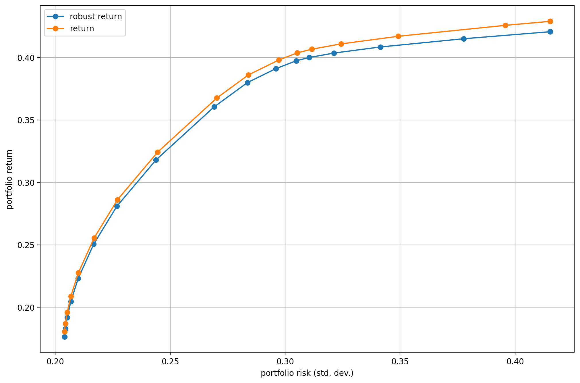
Fig. 10.1 The efficient frontier.

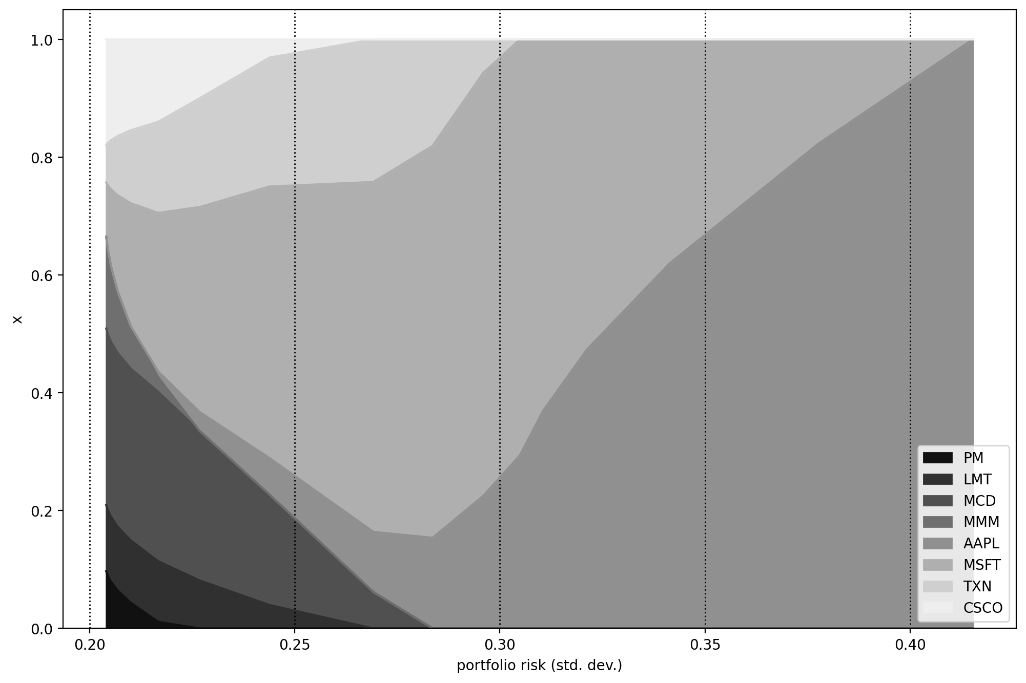
Fig. 10.2 Portfolio composition $\mathbf{x}$ with varying level if risk-aversion $\delta$.

Footnotes

[1]

In the distribution $\mathrm{\Gamma }(a,b)$, $a$ is the shape parameter and $b$ is the rate parameter.

[2]

There is a unique solution because the right-hand side of (10.16) is monotonic on $[0,1]$, and takes values also in $[0,1]$.

[3]

Assuming $K=40$ factors, having $T\ge 50$ data samples allows for a confidence level of ${\omega }^K\ge 0.995$.