7 Benchmark relative portfolio optimization

We often measure the performance of portfolios relative to a benchmark. The benchmark is typically a market index representing an asset class or some segment of the market, and its composition is assumed known. Benchmark relative portfolio management can have two types of strategies: active or passive. The passive strategy tries to replicate the benchmark, i. e. match its performance as closely as possible. In contrast, active management seeks to consistently beat (outperform) the benchmark (after management fees). This section is based on [CJPT18].

7.1 Active return

Let the portfolio and benchmark weights be \(\mathbf{x}\) and \(\mathbf{x}_\mathrm{bm}\). In active management, quantities of interest are the return and the risk relative to the benchmark. The active portfolio return (return above the benchmark return) is

\[R_{\mathbf{x}_\mathrm{a}} = \mathbf{x}_\mathrm{a}^\mathsf{T}R = \mathbf{x}^\mathsf{T}R - \mathbf{x}_\mathrm{bm}^\mathsf{T}R = R_\mathbf{x} - R_{\mathbf{x}_\mathrm{bm}},\]

where \(\mathbf{x}_\mathrm{a} = \mathbf{x} - \mathbf{x}_\mathrm{bm}\) is the active holdings of the portfolio.

The active portfolio risk or tracking error will be the standard deviation of active return:

\[\sigma_{\mathbf{x}_\mathrm{a}}(R_{\mathbf{x}}, R_{\mathbf{x}_\mathrm{bm}}) = \sqrt{\mathbf{x}_\mathrm{a}^\mathsf{T}\Sigma\mathbf{x}_\mathrm{a}},\]

where \(\Sigma\) is the covariance matrix of return. The tracking error measures how close the portfolio return is to the benchmark return. Outperforming the benchmark involves additional risk; if the tracking error is zero then there cannot be any active return at all.

In general we can construct a class of functions for the purpose of measuring tracking error differently, from any deviation measure. See in Sec. 8 (Other risk measures).

7.2 Factor model on active returns

In the active return there is still a systematic component attributable to the benchmark. We can account for that using a single factor model. First we create a factor model for security returns:

\[R = \beta R_{\mathbf{x}_\mathrm{bm}} + \theta,\]

where \(\beta_i = \mathrm{Cov}(R_i, R_{\mathbf{x}_\mathrm{bm}}) / \mathrm{Var}(R_{\mathbf{x}_\mathrm{bm}})\) is the exposure of security \(i\) to the benchmark, \(\mathrm{Cov}(\theta) = \mathbf{0}\), \(\mathrm{Cov}(R_{\mathbf{x}_\mathrm{bm}}, \theta_i) = 0\), and \(\mathbb{E}(\theta_i) = \alpha_i\) is the expected residual return. Under this model, the covariance matrix of \(R\) will be

\[\Sigma = \beta^\mathsf{T}\beta\sigma_{\mathbf{x}_\mathrm{bm}}^2 + \Sigma_\theta,\]

where \(\sigma_{\mathbf{x}_\mathrm{bm}}^2\) is the benchmark variance and \(\Sigma_\theta\) is the residual covariance matrix.

This factor model allows us to decompose the portfolio return into a systematic component, which is explained by the benchmark, and a residual component, which is specific to the portfolio:

\[R_\mathbf{x} = \beta_\mathbf{x} R_{\mathbf{x}_\mathrm{bm}} + \theta_\mathbf{x},\]

where \(\beta_\mathbf{x} = \beta^\mathsf{T}\mathbf{x}\), \(\theta_\mathbf{x} = \theta^\mathsf{T}\mathbf{x}\), and \(\alpha_\mathbf{x} = \alpha^\mathsf{T}\mathbf{x} = \mathbb{E}(\theta_\mathbf{x})\).

Finally, by subtracting the benchmark return from both sides we can write the active return as:

\[R_{\mathbf{x}_\mathrm{a}} = (\beta_\mathbf{x} - 1) R_{\mathbf{x}_\mathrm{bm}} + \theta_\mathbf{x},\]

where \(\beta_\mathbf{x} - 1\) is the active beta. After computing the variance of the decomposed active return, we can also write the square of the tracking error as

\[\sigma^2_{\mathbf{x}_\mathrm{a}}(R_\mathbf{x}, R_{\mathbf{x}_\mathrm{bm}}) = (\beta_\mathbf{x} - 1)^2\sigma_{\mathbf{x}_\mathrm{bm}}^2 + \omega_\mathbf{x}^2,\]

where \(\sigma_{\mathbf{x}_\mathrm{bm}}^2 = \mathrm{Var}(R_{\mathbf{x}_\mathrm{bm}})\), and \(\omega_\mathbf{x}^2 = \mathrm{Var}(\theta_\mathbf{x})\) is the residual risk.

We must note that if a different factor model is used to forecast risk and alpha (which is often the case in practice), there could be factors included in one model but not included in the other model. The optimizer will interpret such misalignments as factor return without risk or factor risk without return and it will exploit them as false opportunities, leading to unintended biases in the results. Risk and alpha factors are considered aligned if alpha can be written as a linear combination of the risk factors. In case of a misalignment, there are different approaches to mitigate it [KS13].

7.3 Optimization

An active investment strategy would try to gain higher portfolio alpha \(\alpha_\mathbf{x}\) at the cost of accepting a higher tracking error. It follows that portfolio optimization with respect to a benchmark will optimize the tradeoff between portfolio alpha and the square of the tracking error. Additional constrains specific to such problems can be bounds on the portfolio active beta or on the active holdings. We can see examples in the following model:

(7.1)\[\begin{split}\begin{array}{lrcl} \mbox{maximize} & \EAlpha^\mathsf{T}\mathbf{x} & &\\ \mbox{subject to} & (\mathbf{x}-\mathbf{x}_\mathrm{bm})^\mathsf{T} \ECov (\mathbf{x}-\mathbf{x}_\mathrm{bm}) & \leq & \gamma_\mathrm{TE}^2,\\ & \mathbf{x}-\mathbf{x}_\mathrm{bm} & \geq & \mathbf{l}_\mathrm{h},\\ & \mathbf{x}-\mathbf{x}_\mathrm{bm} & \leq & \mathbf{u}_\mathrm{h},\\ & \EBeta_\mathbf{x} - 1 & \geq & \mathbf{l}_\beta,\\ & \EBeta_\mathbf{x} - 1 & \leq & \mathbf{u}_\beta,\\ & \mathbf{x} & \in & \mathcal{F}, \end{array}\end{split}\]

where \(\EAlpha\) and \(\EBeta\) are estimates of \(\alpha\) and \(\beta\). To compute these estimates, we can do a linear regression. However, this tends to overestimate the betas of stocks with high benchmark exposure and underestimate the betas of the stocks with low benchmark exposure. To improve the estimation, shrinkage towards one (the beta of the benchmark) can be helpful:

\[\EBeta_\mathrm{shrunk} = (1-c)\EBeta + c\mathbf{1},\]

where we must estimate the optimal shrinkage factor \(c\).

7.4 Extensions

7.4.1 Variance constraint

Optimization of alpha with constraining only the tracking error can increase total portfolio risk. According to [Jor04] it can be helpful to constrain also the total portfolio variance, especially in cases when the benchmark portfolio is relatively inefficient:

(7.2)\[\begin{split}\begin{array}{lrcl} \mbox{maximize} & \EAlpha^\mathsf{T}\mathbf{x} & &\\ \mbox{subject to} & (\mathbf{x}-\mathbf{x}_\mathrm{bm})^\mathsf{T} \ECov (\mathbf{x}-\mathbf{x}_\mathrm{bm}) & \leq & \gamma_\mathrm{TE}^2,\\ & \mathbf{x}^\mathsf{T} \ECov \mathbf{x} & \leq & \gamma^2,\\ & \mathbf{x} & \in & \mathcal{F}. \end{array}\end{split}\]

7.4.2 Passive management

In the case of passive management, the goal of optimization is to construct a benchmark tracking portfolio, i. e., to have a tracking error as small as possible, given the constraints. This usually also means that \(\alpha_\mathbf{x}=0\). Of course without constraints or trading costs, the optimal solution is the benchmark index. Therefore optimization in passive management may only be useful when constraints are needed or liquidity issues are important [MM08].

7.4.3 Linear tracking error measures

The tracking error is one possible measure of closeness between the portfolio and the benchmark. However, there can be other measures [RWZ99]. For example, we can use the mean absolute deviation (MAD) measure, i. e., \(\mathbb{E}(|R_\mathbf{x} - R_{\mathbf{x}_\mathrm{bm}}|)\). Advantage of this measure is its better robustness against outliers in the data. Applying scenario approximation to the expectation we get \(\frac{1}{T}\sum_{k=1}^T\left|\mathbf{r}_k^\mathsf{T}(\mathbf{x}-\mathbf{x}_\mathrm{bm})\right|\). After modeling the absolute value function (see Sec. 13.1.1.3 (Absolute value)), we can formulate the benchmark tracking problem with this measure as an LO model:

(7.3)\[\begin{split}\begin{array}{lrcl} \mbox{maximize}_{\mathbf{x}, \mathbf{t}} & \alpha^\mathsf{T}\mathbf{x} & &\\ \mbox{subject to} & \frac{1}{T}\sum_{k=1}^T t_k & \leq & \gamma,\\ & \mathbf{t} + \mathbf{R}^\mathsf{T} (\mathbf{x}-\mathbf{x}_\mathrm{bm}) & \geq & 0,\\ & \mathbf{t} - \mathbf{R}^\mathsf{T} (\mathbf{x}-\mathbf{x}_\mathrm{bm}) & \geq & 0,\\ & \mathbf{x} & \in & \mathcal{F}, \end{array}\end{split}\]

where \(\mathbf{R}\) is the return data matrix with one observation \(\mathbf{r}_k,\ k = 1,\dots,T\) in each column.

If the investor perceives risk as portfolio return being below the benchmark return, we can also use downside deviation measures. One example is the lower partial moment \(\mathrm{LPM}_1\) measure: \(\mathbb{E}\left(\mathrm{max}(- R_\mathbf{x} + R_{\mathbf{x}_\mathrm{bm}}, 0)\right)\). The scenario approximation of this expectation will be \(\frac{1}{T}\sum_{k=1}^T\mathrm{max}\left(-\mathbf{r}_k^\mathsf{T}(\mathbf{x} -\mathbf{x}_\mathrm{bm}), 0\right)\). After modeling the maximum (see Sec. 13.1.1.1 (Maximum function)) by defining a new variable \(t_k^- = \mathrm{max}\left(-\mathbf{r}_k^\mathsf{T}(\mathbf{x} -\mathbf{x}_\mathrm{bm}), 0\right)\), we can solve the problem as an LO:

(7.4)\[\begin{split}\begin{array}{lrcl} \mbox{maximize} & \alpha^\mathsf{T}\mathbf{x} & &\\ \mbox{subject to} & \frac{1}{T}\sum_{k=1}^T t_k^- & \leq & \gamma,\\ & \mathbf{t}^- & \geq & -\mathbf{R}^\mathsf{T} (\mathbf{x}-\mathbf{x}_\mathrm{bm}),\\ & \mathbf{t}^- & \geq & 0,\\ & \mathbf{x} & \in & \mathcal{F}. \end{array}\end{split}\]

Note that for a symmetric portfolio return distribution, this will be equivalent to the MAD model.

Linear models might be also preferable because of their more intuitive interpretation. By measuring the tracking error according to a linear function, the measurement unit of the objective function is percentage instead of squared percentage.

7.5 Example

Here we show an example of a benchmark relative optimization problem. The benchmark will be the equally weighted portfolio of the eight stocks from the previous examples, therefore \(\mathbf{x}_\mathrm{bm} = \mathbf{1}/N\). The benchmark is created by the following code by aggregating the price data of the eight stocks:

# Create benchmark
df_prices['bm'] = df_prices.iloc[:-2, 0:8].mean(axis=1)

Then we follow the same Monte Carlo procedure as in Sec. 5.5.1 (Single factor model), just with the benchmark instead of the market factor. This will yield scenarios of linear returns on the investment time horizon of \(h=1\) year, so that we can compute estimates \(\EAlpha\) and \(\EBeta\) of \(\alpha\) and \(\beta\) using time-series regression.

In the Fusion model, we make the following modifications:

• We define the active holdings variable \(\mathbf{x}_\mathrm{a} = \mathbf{x} - \mathbf{x}_\mathrm{bm}\) by

  # Active holdings
  xa = x - xbm
  

• We modify the constraint on risk to be the constraint on tracking error:

  # Conic constraint for the portfolio variance
  M.constraint('risk', Expr.vstack(s, 1, G.T @ xa),
               Domain.inRotatedQCone())
  

• We also specify bounds on the active holdings and on the portfolio active beta:

  # Constraint on active holdings
  M.constraint('bound-h', xa, Domain.inRange(lh, uh))
  
  # Constraint on portfolio active beta
  port_act_beta = x.T @ B - 1
  M.constraint('bound-b', port_act_beta, Domain.inRange(lb, ub))
  

• Finally, we modify the objective to maximize the portfolio alpha:

  # Objective (quadratic utility version)
  delta = M.parameter()
  M.objective('obj', ObjectiveSense.Maximize, x.T @ a - delta * s)
  

The complete Fusion model of the optimization problem (7.1) will then be

def EfficientFrontier(N, a, B, G, xbm, deltas, uh, ub, lh, lb):
    with Model("Frontier") as M:
        # Variables
        # The variable x is the fraction of holdings in each security.
        # Non-negative, no short-selling
        x = M.variable("x", N, Domain.greaterThan(0.0))

        # Active holdings
        xa = x - xbm

        # Portfolio variance term in the objective.
        s = M.variable("s", 1, Domain.unbounded())

        # Budget constraint
        M.constraint('budget_x', Expr.sum(x) == 1.0)

        # Constraint on active holdings
        M.constraint('bound-h', xa, Domain.inRange(lh, uh))

        # Constraint on portfolio active beta
        port_act_beta = x.T @ B - 1
        M.constraint('bound-b', port_act_beta, Domain.inRange(lb, ub))

        # Conic constraint for the portfolio variance
        M.constraint('risk', Expr.vstack(s, 1, G.T @ xa),
                             Domain.inRotatedQCone())

        # Objective (quadratic utility version)
        delta = M.parameter()
        M.objective('obj', ObjectiveSense.Maximize, x.T @ a - delta * s)

        # Create DataFrame to store the results. SPY is removed.
        columns = ["delta", "obj", "return", "risk"] + \
                  df_prices.columns[:-1].tolist()
        df_result = pd.DataFrame(columns=columns)
        for d in deltas:
            # Update parameter
            delta.setValue(d);

            # Solve optimization
            M.solve()

            # Save results
            portfolio_return = a @ x.level()
            portfolio_risk = np.sqrt(2 * s.level()[0])
            row = pd.Series([d, M.primalObjValue(), portfolio_return,
                             portfolio_risk] + \
                             list(x.level()), index=columns)
            df_result = pd.concat([df_result, row.to_frame().T],
                                  ignore_index=True)

        return df_result

We give the input parameters and compute the efficient frontier using the following code:

deltas = np.logspace(start=-0.5, stop=2, num=20)[::-1]
xbm = np.ones(N) / N
uh = np.ones(N) * 0.5
lh = -np.ones(N) * 0.5
ub = 0.5
lb = -0.5
df_result = EfficientFrontier(N, a, B, G, xbm, deltas, uh, ub, lh, lb)
mask = df_result < 0
mask.iloc[:, :2] = False
df_result[mask] = 0
df_result

On Fig. 7.1 we plot the efficient frontier and on Fig. 7.2 the portfolio composition. On the latter we see that as the tracking error decreases, the portfolio gets closer to the benchmark, i. e., the equal-weighted portfolio.

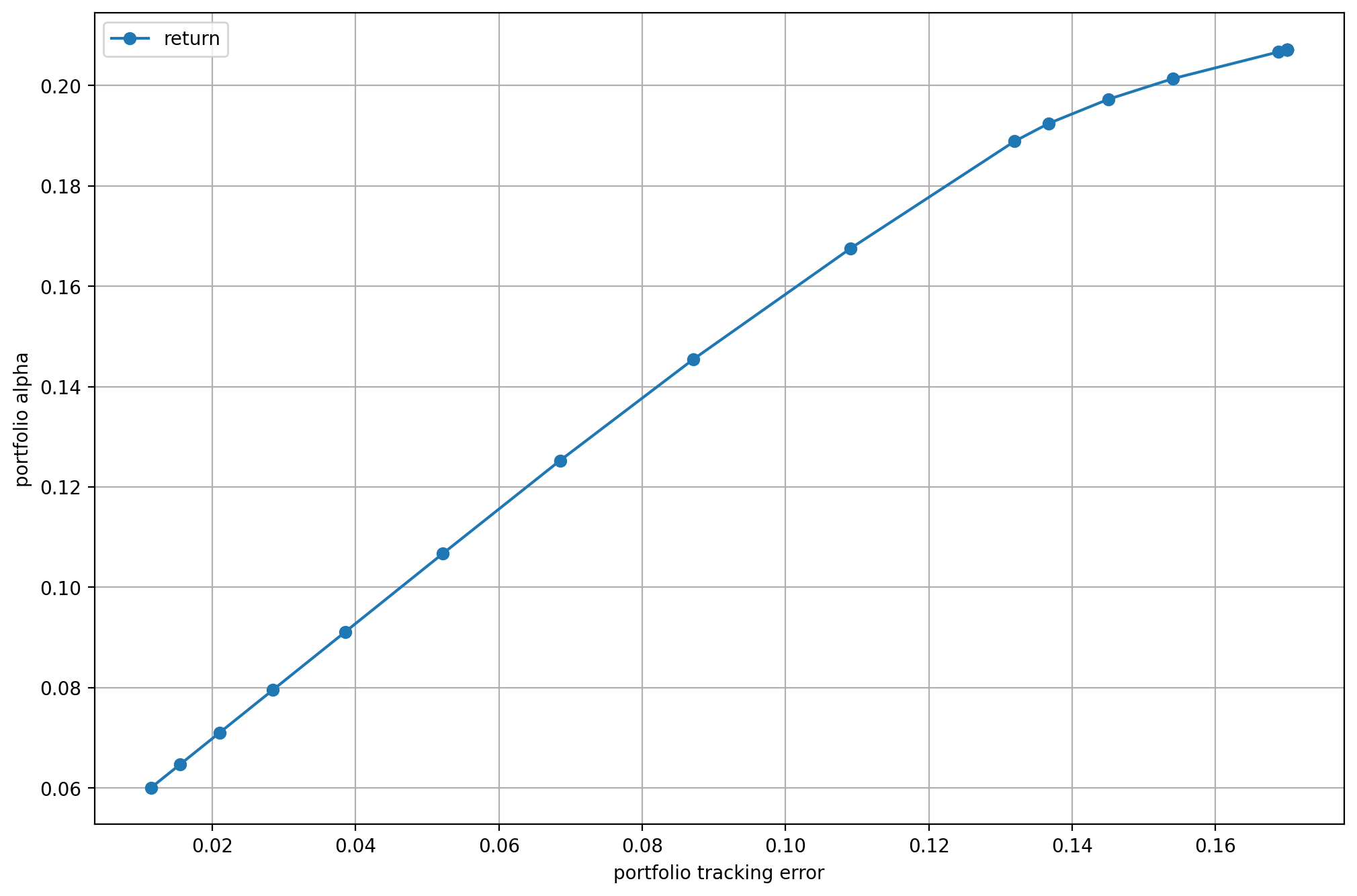
Fig. 7.1 The benchmark relative efficient frontier.

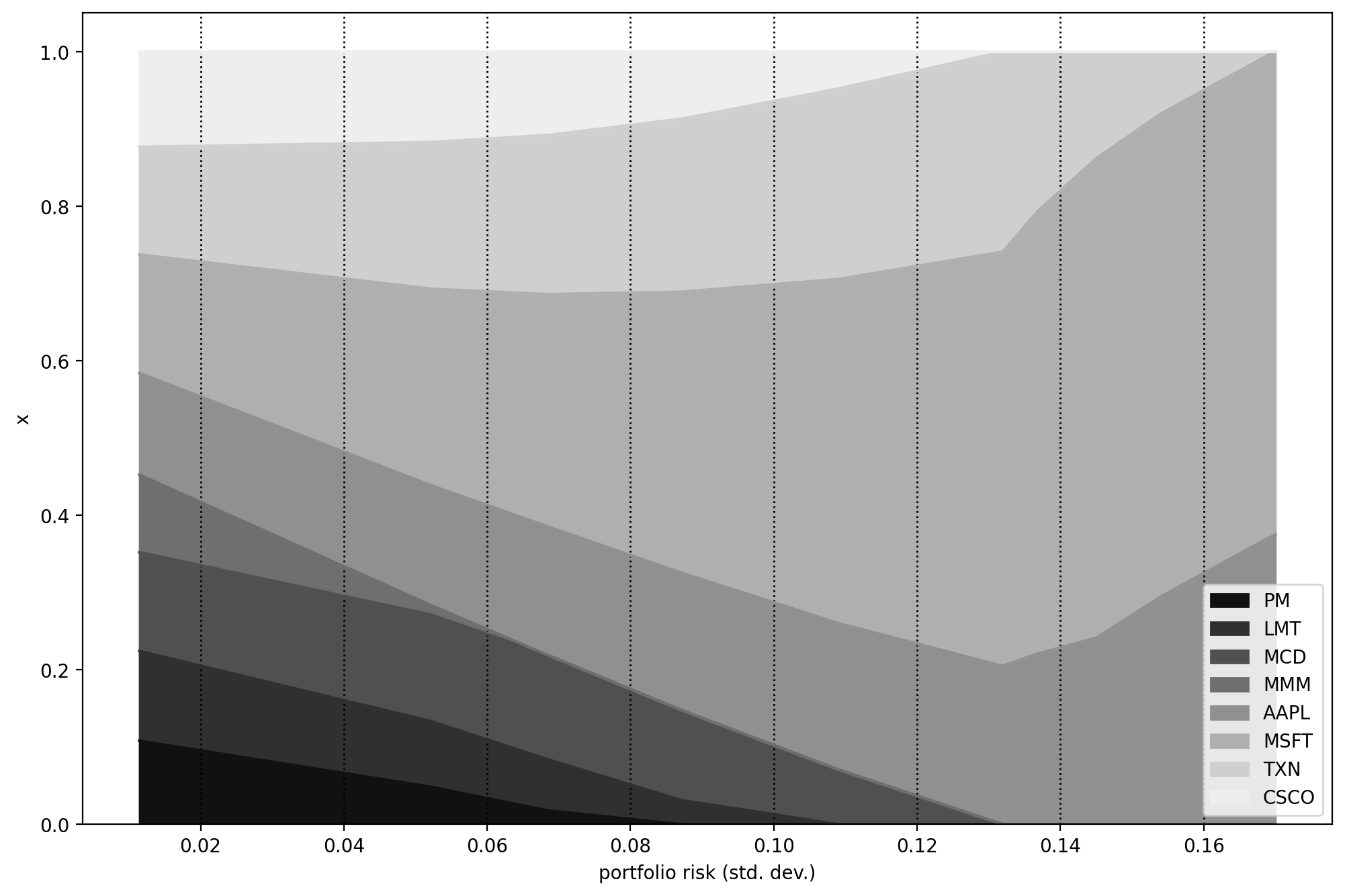
Fig. 7.2 Portfolio composition \(\mathbf{x}\) with varying level if risk-aversion \(\delta\).