11.2 Primal Support-Vector Machine (SVM)
Machine-Learning (ML) has become a common widespread tool in many applications that affect our everyday life. In many cases, at the very core of these techniques there is an optimization problem. This case study focuses on the Support-Vector Machines (SVM).
The basic SVM model can be stated as:
We are given a set of \(m\) points in \(\R^n\), partitioned into two groups. Find, if any, the separating hyperplane of the two subsets with the largest margin, i.e. as far as possible from the points.
Mathematical Model
Let \(x_1,\ldots,x_m\in \R^n\) be the given training set and let \(y_i\in \{-1,+1\}\) be the labels indicating the group membership of the \(i\)-th training example. Then we want to determine an affine hyperplane \(w^T x = b\) that separates the group in the strong sense that
for all \(i\), the property referred to as large margin classification: the strip \(\{x\in\R^n~:~-1<w^Tx-b<1\}\) does not contain any training example. The width of this strip is \(2\|w\|^{-1}\), and maximizing that quantity is equivalent to minimizing \(\|w\|\). We get that the large margin classification is the solution of the following optimization problem:
If a solution exists, \(w,b\) define the separating hyperplane and the sign of \(w^Tx -b\) can be used to decide the class in which a point \(x\) falls.
To allow more flexibility the soft-margin SVM classifier is often used instead. It admits a violation of the large margin requirement (11.13) by a non-negative slack variable which is then penalized in the objective function.
In matrix form we have
where \(\star\) denotes the component-wise product, and \(\mathbf{e}\) a vector with all components equal to one. The constant \(C\geq 0\) acts both as scaling factor and as weight. Varying \(C\) yields different trade-offs between accuracy and robustness.
Implementing the matrix formulation of the soft-margin SVM in Fusion is very easy. We only need to cast the problem in conic form, which in this case involves converting the quadratic term of the objective function into a conic constraint:
where \(\Qr^{n+2}\) denotes a rotated cone of dimension \(n+2\).
Fusion implementation
We now demonstrate how implement model (11.14). Let us assume that the training examples are stored in the rows of a matrix X, the labels in a vector y and that we have a set of weights C for which we want to train the model. The implementation in Fusion of our conic model starts declaring the model class:
Model::t M = new Model("primal SVM"); auto _M = finally([&]() { M->dispose(); });
Then we proceed defining the variables :
  Variable::t w  =  M->variable( n, Domain::unbounded());
  Variable::t t  =  M->variable( 1, Domain::unbounded());
  Variable::t b  =  M->variable( 1, Domain::unbounded());
  Variable::t xi =  M->variable( m, Domain::greaterThan(0.));
The conic constraint is obtained by stacking the three values:
M->constraint( Expr::vstack(1., t, w) , Domain::inRotatedQCone() );
Note how the dimension of the cone is deduced from the arguments. The relaxed classification constraints can be expressed using the built-in expressions available in Fusion. In particular:
element-wise multiplication \(\star\) is performed with the
Expr.mulElmfunction;a vector whose entries are repetitions of \(b\) is produced by
Var.repeat.
The results is
  auto ex = Expr::sub( Expr::mul(X, w), Var::repeat(b, m) );
  M->constraint( Expr::add(Expr::mulElm( y, ex ), xi ) , Domain::greaterThan( 1. ) );
Finally, the objective function is defined as
M->objective( ObjectiveSense::Minimize, Expr::add( t, Expr::mul(c, Expr::sum(xi) ) ) );
To solve a sequence of problems with varying C we can simply iterate along those values changing the objective function:
  std::cout << "   c   | b      | w\n";
  for (int i = 0; i < nc; i++)
  {
    double c = 500.0 * i;
    M->objective( ObjectiveSense::Minimize, Expr::add( t, Expr::mul(c, Expr::sum(xi) ) ) );
    M->solve();

    try
    {
      std::cout << std::setw(6) << c << " | " << std::setw(8) << (*(b->level())) [0] << " | ";
      std::cout.width(8);
      auto wlev = w->level();
      std::copy( wlev->begin(), wlev->end() , std::ostream_iterator<double>(std::cout, " ") );
      std::cout << "\n";
    }
    catch (...) {}

  }
Source code
  Model::t M = new Model("primal SVM"); auto _M = finally([&]() { M->dispose(); });

  Variable::t w  =  M->variable( n, Domain::unbounded());
  Variable::t t  =  M->variable( 1, Domain::unbounded());
  Variable::t b  =  M->variable( 1, Domain::unbounded());
  Variable::t xi =  M->variable( m, Domain::greaterThan(0.));

  auto ex = Expr::sub( Expr::mul(X, w), Var::repeat(b, m) );
  M->constraint( Expr::add(Expr::mulElm( y, ex ), xi ) , Domain::greaterThan( 1. ) );

  M->constraint( Expr::vstack(1., t, w) , Domain::inRotatedQCone() );

  std::cout << "   c   | b      | w\n";
  for (int i = 0; i < nc; i++)
  {
    double c = 500.0 * i;
    M->objective( ObjectiveSense::Minimize, Expr::add( t, Expr::mul(c, Expr::sum(xi) ) ) );
    M->solve();

    try
    {
      std::cout << std::setw(6) << c << " | " << std::setw(8) << (*(b->level())) [0] << " | ";
      std::cout.width(8);
      auto wlev = w->level();
      std::copy( wlev->begin(), wlev->end() , std::ostream_iterator<double>(std::cout, " ") );
      std::cout << "\n";
    }
    catch (...) {}

  }
Example
We generate a random dataset consisting of two groups of points, each from a Gaussian distribution in \(\R^2\) with centres \((1.0,1.0)\) and \((-1.0,-1.0)\), respectively.
  int m = 50 ;
  int n = 3;
  int nc = 10;

  int nump = m / 2;
  int numm = m - nump;

  auto y = new_array_ptr<double, 1> (m);
  std::fill( y->begin(), y->begin() + nump, 1.);
  std::fill( y->begin() + nump, y->end(), -1.);

  double mean = 1.;
  double var = 1.;

  auto X = std::shared_ptr< ndarray<double, 2> > (  new ndarray<double, 2> ( shape_t<2>(m, n) ) );

  std::mt19937 e2(0);

  for (int i = 0; i < nump; i++)
  {
    auto ram = std::bind(std::normal_distribution<>(mean, var), e2);
    for ( int j = 0; j < n; j++)
      (*X)(i, j) = ram();
  }

  std::cout << "Number of data    : " << m << std::endl;
  std::cout << "Number of features: " << n << std::endl;
With standard deviation \(\sigma= 1/2\) we obtain a separable instance of the problem with a solution shown in Fig. 11.2.
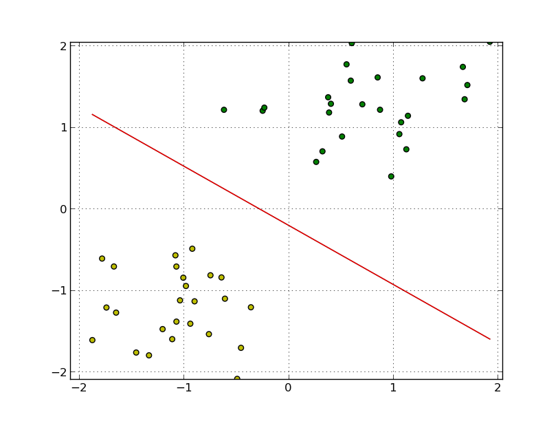
Fig. 11.2 Separating hyperplane for two clusters of points.
For \(\sigma=1\) the two groups are not linearly separable and the we obtain the optimal hyperplane as in Fig. 11.3.

Fig. 11.3 Soft separating hyperplane for two groups of points.