11.5 Logistic regression

Logistic regression is an example of a binary classifier, where the output takes one two values 0 or 1 for each data point. We call the two values classes.

Formulation as an optimization problem

Define the sigmoid function

$$S(x)=\frac{1}{1+\exp (-x)}.$$

Next, given an observation $x\in {\mathbb{R}}^d$ and a weights $\theta \in {\mathbb{R}}^d$ we set

$$h_{\theta }(x)=S({\theta }^{T}x)=\frac{1}{1+\exp (-{\theta }^{T}x)}.$$

The weights vector $\theta$ is part of the setup of the classifier. The expression $h_{\theta }(x)$ is interpreted as the probability that $x$ belongs to class 1. When asked to classify $x$ the returned answer is

$$\begin{array}{r}x\mapsto \{\begin{array}{l}\begin{array}{ll}1& h_{\theta }(x)\ge 1/2,\\ 0& h_{\theta }(x)<1/2.\end{array}\end{array}\end{array}$$

When training a logistic regression algorithm we are given a sequence of training examples $x_i$, each labelled with its class $y_i\in \{0,1\}$ and we seek to find the weights $\theta$ which maximize the likelihood function

$$\prod _i{h}_{\theta }(x_i{)}^{y_i}(1-h_{\theta }(x_i){)}^{1-y_i}.$$

Of course every single $y_i$ equals 0 or 1, so just one factor appears in the product for each training data point. By taking logarithms we can define the logistic loss function:

$$J(\theta )=-\sum _{i:y_i=1}\log (h_{\theta }(x_i))-\sum _{i:y_i=0}\log (1-h_{\theta }(x_i)).$$

The training problem with regularization (a standard technique to prevent overfitting) is now equivalent to

$$\underset{\theta }{min}J(\theta )+\lambda \Vert \theta {\Vert }_2.$$

This can equivalently be phrased as

(11.20)$$\begin{array}{r}\begin{array}{lrllr}\text{minimize}& \sum _i{t}_i+\lambda r& & & \\ \text{subject to}& t_i& \ge -\log (h_{\theta }(x))& =\log (1+\exp (-{\theta }^T{x}_i))& \mathrm{if}{y}_i=1,\\ & t_i& \ge -\log (1-h_{\theta }(x))& =\log (1+\exp ({\theta }^T{x}_i))& \mathrm{if}{y}_i=0,\\ & r& \ge \Vert \theta {\Vert }_2.& & \end{array}\end{array}$$

Implementation

As can be seen from (11.20) the key point is to implement the softplus bound $t\ge \log (1+e^u)$, which is the simplest example of a log-sum-exp constraint for two terms. Here $t$ is a scalar variable and $u$ will be the affine expression of the form $\pm {\theta }^T{x}_i$. This is equivalent to

$$\exp (u-t)+\exp (-t)\le 1$$

and further to

(11.21)$$\begin{array}{r}\begin{array}{rclr}(z_1,1,u-t)& \in & K_{\exp }& (z_1\ge \exp (u-t)),\\ (z_2,1,-t)& \in & K_{\exp }& (z_2\ge \exp (-t)),\\ z_1+z_2& \le & 1.& \end{array}\end{array}$$

Listing 11.11 Implementation of $t\ge \log (1+e^u)$ as in (11.21). Click here to download.

// t >= log( 1 + exp(u) ) coordinatewise
void softplus(Model::t      M,
              Expression::t t,
              Expression::t u)
{
    int n = (*t->getShape())[0];
    auto z1 = M->variable(n);
    auto z2 = M->variable(n);
    M->constraint(Expr::add(z1, z2), Domain::equalsTo(1));
    M->constraint(Expr::hstack(z1, Expr::constTerm(n, 1.0), Expr::sub(u,t)), Domain::inPExpCone());
    M->constraint(Expr::hstack(z2, Expr::constTerm(n, 1.0), Expr::neg(t)), Domain::inPExpCone());
}

Once we have this subroutine, it is easy to implement a function that builds the regularized loss function model (11.20).

Listing 11.12 Implementation of (11.20). Click here to download.

// Model logistic regression (regularized with full 2-norm of theta)
// X - n x d matrix of data points
// y - length n vector classifying training points
// lamb - regularization parameter
std::pair<Model::t, Variable::t>
logisticRegression(std::vector<std::vector<double>> & X, 
                   std::vector<bool>                & y,
                   double                           lamb)
{
    int n = X.size();
    int d = X[0].size();       // num samples, dimension
    
    Model::t M = new Model();   

    auto theta = M->variable(d);
    auto t     = M->variable(n);
    auto reg   = M->variable();

    M->objective(ObjectiveSense::Minimize, Expr::add(Expr::sum(t), Expr::mul(lamb,reg)));
    M->constraint(Var::vstack(reg, theta), Domain::inQCone());

    auto signs = std::make_shared<ndarray<double,1>>(shape(n), [y](ptrdiff_t i) { return y[i] ? -1 : 1; });   

    softplus(M, t, Expr::mulElm(Expr::mul(new_array_ptr<double>(X), theta), signs));

    return std::make_pair(M, theta);
}

Example: 2D dataset fitting

In the next figure we apply logistic regression to the training set of 2D points taken from the example ex2data2.txt . The two-dimensional dataset was converted into a feature vector $x\in {\mathbb{R}}^{28}$ using monomial coordinates of degrees at most 6.

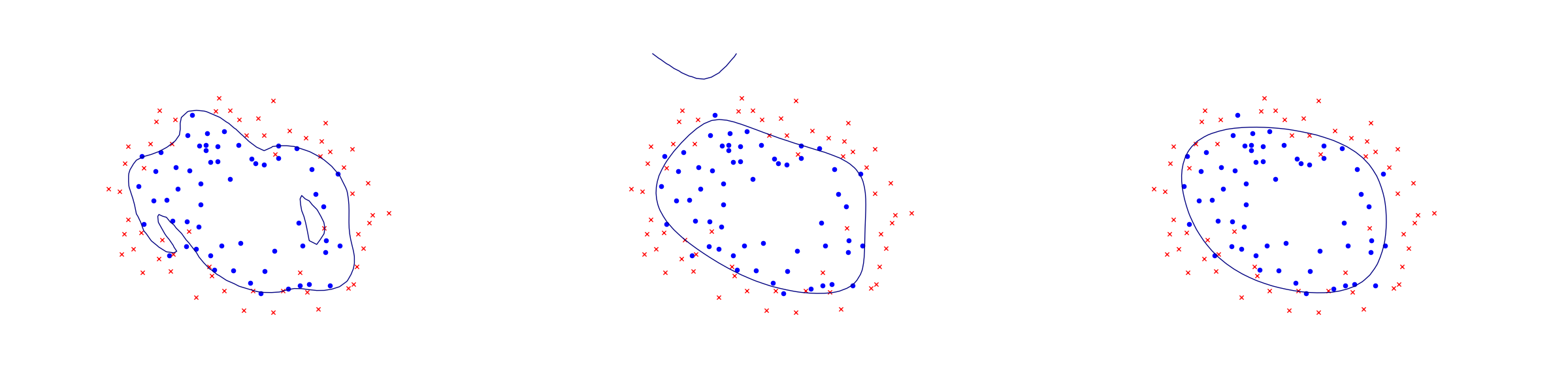
Fig. 11.6 Logistic regression example with none, medium and strong regularization (small, medium, large $\lambda$). Without regularization we get obvious overfitting.