11.6 Inner and outer Löwner-John Ellipsoids
In this section we show how to compute the Löwner-John inner and outer ellipsoidal approximations of a polytope. They are defined as, respectively, the largest volume ellipsoid contained inside the polytope and the smallest volume ellipsoid containing the polytope, as seen in Fig. 11.7.
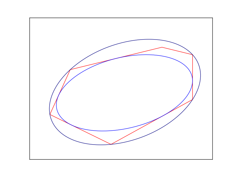
Fig. 11.7 The inner and outer Löwner-John ellipse of a polygon.
For further mathematical details, such as uniqueness of the two ellipsoids, consult [BenTalN01]. Our solution is a mix of conic and semidefinite programming. Among other things, in Sec. 11.6.3 (Bound on the Determinant Root) we show how to implement bounds involving the determinant of a PSD matrix.
11.6.1 Inner Löwner-John Ellipsoids
Suppose we have a polytope given by an h-representation
and we wish to find the inscribed ellipsoid with maximal volume. It will be convenient to parametrize the ellipsoid as an affine transformation of the standard disk:
Every non-degenerate ellipsoid has a parametrization such that \(C\) is a positive definite symmetric \(n\times n\) matrix. Now the volume of \(\mathcal{E}\) is proportional to \(\mbox{det}(C)^{1/n}\). The condition \(\mathcal{E}\subseteq\mathcal{P}\) is equivalent to the inequality \(A(Cu+d)\leq b\) for all \(u\) with \(\|u\|_2\leq 1\). After a short computation we obtain the formulation:
where \(X_i\) denotes the \(i\)-th row of the matrix \(X\). This can easily be implemented using Fusion, where the sequence of conic inequalities can be realized at once by feeding in the matrices \(b-Ad\) and \(AC\).
std::pair<std::shared_ptr<ndarray<double, 1>>, std::shared_ptr<ndarray<double, 1>>>
    lownerjohn_inner
    ( std::shared_ptr<ndarray<double, 2>> A,
      std::shared_ptr<ndarray<double, 1>> b)
{
  Model::t M = new Model("lownerjohn_inner"); auto _M = finally([&]() { M->dispose(); });
  int m = A->size(0);
  int n = A->size(1);

  // Setup variables
  Variable::t t = M->variable("t", 1, Domain::greaterThan(0.0));
  Variable::t C = det_rootn(M, t, n);
  Variable::t d = M->variable("d", n, Domain::unbounded());

  // quadratic cones
  M->constraint(Expr::hstack(Expr::sub(b, Expr::mul(A, d)), Expr::mul(A, C)),
                Domain::inQCone());

  // Objective: Maximize t
  M->objective(ObjectiveSense::Maximize, t);
  M->solve();

  return std::make_pair(C->level(), d->level());
}
The only black box is the method det_rootn which implements the constraint \(t\leq \mbox{det}(C)^{1/n}\). It will be described in Sec. 11.6.3 (Bound on the Determinant Root).
11.6.2 Outer Löwner-John Ellipsoids
To compute the outer ellipsoidal approximation to a polytope, let us now start with a v-representation
of the polytope as a convex hull of a set of points. We are looking for an ellipsoid given by a quadratic inequality
whose volume is proportional to \(\mbox{det}(P)^{-1/n}\), so we are after maximizing \(\mbox{det}(P)^{1/n}\). Again, there is always such a representation with a symmetric, positive definite matrix \(P\). The inclusion conditions \(x_i\in\mathcal{E}\) translate into a straightforward problem formulation:
and then directly into Fusion code:
std::pair<std::shared_ptr<ndarray<double, 1>>, std::shared_ptr<ndarray<double, 1>>>
    lownerjohn_outer(std::shared_ptr<ndarray<double, 2>> x)
{
  Model::t M = new Model("lownerjohn_outer");
  int m = x->size(0);
  int n = x->size(1);

  // Setup variables
  Variable::t t = M->variable("t", 1, Domain::greaterThan(0.0));
  Variable::t P = det_rootn(M, t, n);
  Variable::t c = M->variable("c", n, Domain::unbounded());

  // (1, Px-c) \in Q
  M->constraint(Expr::hstack(
                  Expr::ones(m), Expr::sub(Expr::mul(x, P),
                      Var::reshape(Var::repeat(c, m), new_array_ptr<int, 1>({m, n}))) ),
                Domain::inQCone());

  // Objective: Maximize t
  M->objective(ObjectiveSense::Maximize, t);
  M->solve();

  return std::make_pair(P->level(), c->level());
}
11.6.3 Bound on the Determinant Root
It remains to show how to express the bounds on \(\mbox{det}(X)^{1/n}\) for a symmetric positive definite \(n\times n\) matrix \(X\) using PSD and conic quadratic variables. We want to model the set
A standard approach when working with the determinant of a PSD matrix is to consider a semidefinite cone
where \(Z\) is a matrix of additional variables and where we intuitively identify \(\mbox{Diag}(Z)=\{\lambda_1,\ldots,\lambda_n\}\) with the eigenvalues of \(X\). With this in mind, we are left with expressing the constraint
but this is exactly the geometric mean cone Domain.inPGeoMeanCone. We obtain the following model:
Variable::t det_rootn(Model::t M, Variable::t t, int n)
{
  // Setup variables
  Variable::t Y = M->variable(Domain::inPSDCone(2 * n));

  Variable::t X   = Y->slice(new_array_ptr<int,1>({0, 0}), new_array_ptr<int,1>({n, n}));
  Variable::t Z   = Y->slice(new_array_ptr<int,1>({0, n}), new_array_ptr<int,1>({n, 2 * n}));
  Variable::t DZ  = Y->slice(new_array_ptr<int,1>({n, n}), new_array_ptr<int,1>({2 * n, 2 * n}));

  // Z is lower-triangular
  std::shared_ptr<ndarray<int,2>> low_tri( new ndarray<int,2>( shape_t<2>(n*(n-1)/2, 2) ));
  int k = 0;
  for(int i = 0; i < n; i++)
    for(int j = i+1; j < n; j++)
       (*low_tri)(k,0) = i, (*low_tri)(k,1) = j, ++k;
  M->constraint(Z->pick(low_tri), Domain::equalsTo(0.0));
  // DZ = Diag(Z)
  M->constraint(Expr::sub(DZ, Expr::mulElm(Z, Matrix::eye(n))), Domain::equalsTo(0.0));

  // (Z11*Z22*...*Znn) >= t^n
  M->constraint(Expr::vstack(DZ->diag(), t), Domain::inPGeoMeanCone());

  // Return an n x n PSD variable which satisfies t <= det(X)^(1/n)
  return X;
}