6 Semidefinite optimization

In this chapter we extend the conic optimization framework introduced before with symmetric positive semidefinite matrix variables.

6.1 Introduction to semidefinite matrices

6.1.1 Semidefinite matrices and cones

A symmetric matrix $X\in {\mathcal{S}}^n$ is called symmetric positive semidefinite if

$$z^{T}Xz\ge 0,\mathrm{\forall }z\in {\mathbb{R}}^n.$$

We then define the cone of symmetric positive semidefinite matrices as

(6.1)$${\mathcal{S}}_{+}^n=\{X\in {\mathcal{S}}^n\mid z^{T}Xz\ge 0,\mathrm{\forall }z\in {\mathbb{R}}^n\}.$$

For brevity we will often use the shorter notion semidefinite instead of symmetric positive semidefinite, and we will write $X⪰Y$ ($X⪯Y$) as shorthand notation for $(X-Y)\in {\mathcal{S}}_{+}^n$ ($(Y-X)\in {\mathcal{S}}_{+}^n$). As inner product for semidefinite matrices, we use the standard trace inner product for general matrices, i.e.,

$$⟨A,B⟩:=\mathrm{tr}(A^{T}B)=\sum _{ij}{a}_{ij}{b}_{ij}.$$

It is easy to see that (6.1) indeed specifies a convex cone; it is pointed (with origin $X=0$), and $X,Y\in {\mathcal{S}}_{+}^n$ implies that $(\alpha X+\beta Y)\in {\mathcal{S}}_{+}^n,\alpha ,\beta \ge 0$. Let us review a few equivalent definitions of ${\mathcal{S}}_{+}^n$. It is well-known that every symmetric matrix $A$ has a spectral factorization

$$A=\sum _{i=1}^n{\lambda }_i{q}_i{q}_i^T.$$

where $q_i\in {\mathbb{R}}^n$ are the (orthogonal) eigenvectors and ${\lambda }_i$ are eigenvalues of $A$. Using the spectral factorization of $A$ we have

$$x^{T}Ax=\sum _{i=1}^n{\lambda }_i(x^T{q}_i{)}^2,$$

which shows that $x^{T}Ax\ge 0\iff {\lambda }_i\ge 0,i=1,\dots ,n$. In other words,

(6.3)$${\mathcal{S}}_{+}^n=\{X\in {\mathcal{S}}^n\mid {\lambda }_i(X)\ge 0,i=1,\dots ,n\}.$$

Another useful characterization is that $A\in {\mathcal{S}}_{+}^n$ if and only if it is a Grammian matrix $A=V^{T}V$. Here $V$ is called the Cholesky factor of $A$. Using the Grammian representation we have

$$x^{T}Ax=x^T{V}^{T}Vx=\Vert Vx{\Vert }_2^2,$$

i.e., if $A=V^{T}V$ then $x^{T}Ax\ge 0$ for all $x$. On the other hand, from the positive spectral factorization $A=Q\mathrm{\Lambda }{Q}^T$ we have $A=V^{T}V$ with $V={\mathrm{\Lambda }}^{1/2}{Q}^T$, where ${\mathrm{\Lambda }}^{1/2}=\mathbf{Diag}(\sqrt{{\lambda }_1},\dots ,\sqrt{{\lambda }_n})$. We thus have the equivalent characterization

(6.4)$${\mathcal{S}}_{+}^n=\{X\in {\mathcal{S}}_{+}^n\mid X=V^{T}V\text{ for some }V\in {\mathbb{R}}^{n\times n}\}.$$

In a completely analogous way we define the cone of symmetric positive definite matrices as

$$\begin{array}{r}\begin{array}{cl}{\mathcal{S}}_{++}^n& =\{X\in {\mathcal{S}}^n\mid z^{T}Xz>0,\mathrm{\forall }z\in {\mathbb{R}}^n\}\\ & =\{X\in {\mathcal{S}}^n\mid {\lambda }_i(X)>0,i=1,\dots ,n\}\\ & =\{X\in {\mathcal{S}}_{+}^n\mid X=V^{T}V\text{ for some }V\in {\mathbb{R}}^{n\times n},\mathbf{rank}(V)=n\},\end{array}\end{array}$$

and we write $X\succ Y$ ($X\prec Y$) as shorthand notation for $(X-Y)\in {\mathcal{S}}_{++}^n$ ($(Y-X)\in {\mathcal{S}}_{++}^n$).

The one dimensional cone ${\mathcal{S}}_{+}^1$ simply corresponds to ${\mathbb{R}}_{+}$. Similarly consider

$$\begin{array}{r}X=\left[\begin{array}{cc}{x}_1& x_3\\ x_3& x_2\end{array}\right]\end{array}$$

with determinant $det(X)=x_1{x}_2-x_3^2={\lambda }_1{\lambda }_2$ and trace $\mathrm{tr}(X)=x_1+x_2={\lambda }_1+{\lambda }_2$. Therefore $X$ has positive eigenvalues if and only if

$$x_1{x}_2\ge x_3^2,x_1,x_2\ge 0,$$

which characterizes a three-dimensional scaled rotated cone, i.e.,

$$\begin{array}{r}\left[\begin{array}{cc}{x}_1& x_3\\ x_3& x_2\end{array}\right]\in {\mathcal{S}}_{+}^2⟺(x_1,x_2,x_3\sqrt{2})\in {\mathcal{Q}}_r^3.\end{array}$$

More generally we have

$$x\in {\mathbb{R}}_{+}^n⟺\mathbf{Diag}(x)\in {\mathcal{S}}_{+}^n$$

and

$$\begin{array}{r}(t,x)\in {\mathcal{Q}}^{n+1}⟺\left[\begin{array}{cc}t& x^T\\ x& tI\end{array}\right]\in {\mathcal{S}}_{+}^{n+1},\end{array}$$

where the latter equivalence follows immediately from Lemma 6.1. Thus both the linear and quadratic cone are embedded in the semidefinite cone. In practice, however, linear and quadratic cones should never be described using semidefinite constraints, which would result in a large performance penalty by squaring the number of variables.

Example 6.1

As a more interesting example, consider the symmetric matrix

(6.5)$$\begin{array}{r}A(x,y,z)=\left[\begin{array}{ccc}1& x& y\\ x& 1& z\\ y& z& 1\end{array}\right]\end{array}$$

parametrized by $(x,y,z)$. The set

$$S=\{(x,y,z)\in {\mathbb{R}}^3\mid A(x,y,z)\in {\mathcal{S}}_{+}^3\},$$

(shown in Fig. 6.1) is called a spectrahedron and is perhaps the simplest bounded semidefinite representable set, which cannot be represented using (finitely many) linear or quadratic cones. To gain a geometric intuition of $S$, we note that

$$det(A(x,y,z))=-(x^2+y^2+z^2-2xyz-1),$$

so the boundary of $S$ can be characterized as

$$x^2+y^2+z^2-2xyz=1,$$

or equivalently as

$$\begin{array}{r}{\left[\begin{array}{c}x\\ y\end{array}\right]}^T\left[\begin{array}{rr}1& -z\\ -z& 1\end{array}\right]\left[\begin{array}{c}x\\ y\end{array}\right]=1-z^2.\end{array}$$

For $z=0$ this describes a circle in the $(x,y)$-plane, and for $-1\le z\le 1$ it characterizes an ellipse (for a fixed $z$).

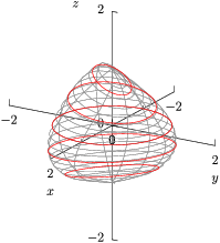
Fig. 6.1 Plot of spectrahedron $S=\{(x,y,z)\in {\mathbb{R}}^3\mid A(x,y,z)⪰0\}$.

6.1.2 Properties of semidefinite matrices

Many useful properties of (semi)definite matrices follow directly from the definitions (6.1)-(6.4) and their definite counterparts.

• The diagonal elements of $A\in {\mathcal{S}}_{+}^n$ are nonnegative. Let $e_i$ denote the $i$th standard basis vector (i.e., $[e_i{]}_j=0,j\ne i$, $[e_i{]}_i=1$). Then $A_{ii}=e_i^{T}A{e}_i$, so (6.1) implies that $A_{ii}\ge 0$.

• A block-diagonal matrix $A=\mathbf{Diag}(A_1,\dots A_p)$ is (semi)definite if and only if each diagonal block $A_i$ is (semi)definite.

• Given a quadratic transformation $M:=B^{T}AB$, $M\succ 0$ if and only if $A\succ 0$ and $B$ has full rank. This follows directly from the Grammian characterization $M=(VB{)}^T(VB)$. For $M⪰0$ we only require that $A⪰0$. As an example, if $A$ is (semi)definite then so is any permutation $P^{T}AP$.

• Any principal submatrix of $A\in {\mathcal{S}}_{+}^n$ ($A$ restricted to the same set of rows as columns) is positive semidefinite; this follows by restricting the Grammian characterization $A=V^{T}V$ to a submatrix of $V$.

• The inner product of positive (semi)definite matrices is positive (nonnegative). For any $A,B\in {\mathcal{S}}_{++}^n$ let $A=U^{T}U$ and $B=V^{T}V$ where $U$ and $V$ have full rank. Then

  $$⟨A,B⟩=\mathrm{tr}(U^{T}U{V}^{T}V)=\Vert U{V}^T{\Vert }_F^2>0,$$

  where strict positivity follows from the assumption that $U$ has full column-rank, i.e., $U{V}^T\ne 0$.

• The inverse of a positive definite matrix is positive definite. This follows from the positive spectral factorization $A=Q\mathrm{\Lambda }{Q}^T$, which gives us

  $$A^{-1}=Q^T{\mathrm{\Lambda }}^{-1}Q$$

  where ${\mathrm{\Lambda }}_{ii}>0$. If $A$ is semidefinite then the pseudo-inverse $A^{†}$ of $A$ is semidefinite.

• Consider a matrix $X\in {\mathcal{S}}^n$ partitioned as

  $$\begin{array}{r}X=\left[\begin{array}{cc}A& B^T\\ B& C\end{array}\right].\end{array}$$

  Let us find necessary and sufficient conditions for $X\succ 0$. We know that $A\succ 0$ and $C\succ 0$ (since any principal submatrix must be positive definite). Furthermore, we can simplify the analysis using a nonsingular transformation

  $$\begin{array}{r}L=\left[\begin{array}{cc}I& 0\\ F& I\end{array}\right]\end{array}$$

  to diagonalize $X$ as $LX{L}^T=D$, where $D$ is block-diagonal. Note that $det(L)=1$, so $L$ is indeed nonsingular. Then $X\succ 0$ if and only if $D\succ 0$. Expanding $LX{L}^T=D$, we get

  $$\begin{array}{r}\left[\begin{array}{cc}A& A{F}^T+B^T\\ FA+B& FA{F}^T+F{B}^T+B{F}^T+C\end{array}\right]=\left[\begin{array}{cc}{D}_1& 0\\ 0& D_2\end{array}\right].\end{array}$$

  Since $det(A)\ne 0$ (by assuming that $A\succ 0$) we see that $F=-B{A}^{-1}$ and direct substitution gives us

  $$\begin{array}{r}\left[\begin{array}{cc}A& 0\\ 0& C-B{A}^{-1}{B}^T\end{array}\right]=\left[\begin{array}{cc}{D}_1& 0\\ 0& D_2\end{array}\right].\end{array}$$

In the last part we have thus established the following useful result.

Lemma 6.1 Schur complement lemma

A symmetric matrix

$$\begin{array}{r}X=\left[\begin{array}{cc}A& B^T\\ B& C\end{array}\right].\end{array}$$

is positive definite if and only if

$$A\succ 0,C-B{A}^{-1}{B}^T\succ 0.$$

6.2 Semidefinite modeling

Having discussed different characterizations and properties of semidefinite matrices, we next turn to different functions and sets that can be modeled using semidefinite cones and variables. Most of those representations involve semidefinite matrix-valued affine functions, which we discuss next.

6.2.1 Linear matrix inequalities

Consider an affine matrix-valued mapping $A:{\mathbb{R}}^n\mapsto {\mathcal{S}}^m$:

(6.8)$$A(x)=A_0+x_1{A}_1+\cdots +x_n{A}_n.$$

A linear matrix inequality (LMI) is a constraint of the form

(6.9)$$A_0+x_1{A}_1+\cdots +x_n{A}_n⪰0$$

in the variable $x\in {\mathbb{R}}^n$ with symmetric coefficients $A_i\in {\mathcal{S}}^m,i=0,\dots ,n$. As a simple example consider the matrix in (6.5),

$$A(x,y,z)=A_0+x{A}_1+y{A}_2+z{A}_3⪰0$$

with

$$\begin{array}{r}\begin{array}{cccc}{A}_0=I,& A_1=\left[\begin{array}{ccc}0& 1& 0\\ 1& 0& 0\\ 0& 0& 0\end{array}\right],& A_2=\left[\begin{array}{ccc}0& 0& 1\\ 0& 0& 0\\ 1& 0& 0\end{array}\right],& A_3=\left[\begin{array}{ccc}0& 0& 0\\ 0& 0& 1\\ 0& 1& 0\end{array}\right].\end{array}\end{array}$$

Alternatively, we can describe the linear matrix inequality $A(x,y,z)⪰0$ as

$$X\in {\mathcal{S}}_{+}^3,X_{11}=X_{22}=X_{33}=1,x=X_{21},y=X_{31},z=X_{32},$$

i.e., as a semidefinite variable with fixed diagonal; these two alternative formulations illustrate the difference between primal and dual form of semidefinite problems, see Sec. 8.6 (Semidefinite duality and LMIs).

6.2.2 Eigenvalue optimization

Consider a symmetric matrix $A\in {\mathcal{S}}^m$ and let its eigenvalues be denoted by

$${\lambda }_1(A)\ge {\lambda }_2(A)\ge \cdots \ge {\lambda }_m(A).$$

A number of different functions of ${\lambda }_i$ can then be described using a mix of linear and semidefinite constraints.

Sum of eigenvalues

The sum of the eigenvalues corresponds to

$$\sum _{i=1}^m{\lambda }_i(A)=\mathrm{tr}(A).$$

Largest eigenvalue

The largest eigenvalue can be characterized in epigraph form ${\lambda }_1(A)\le t$ as

(6.10)$$tI-A⪰0.$$

To verify this, suppose we have a spectral factorization $A=Q\mathrm{\Lambda }{Q}^T$ where $Q$ is orthogonal and $\mathrm{\Lambda }$ is diagonal. Then $t$ is an upper bound on the largest eigenvalue if and only if

$$Q^T(tI-A)Q=tI-\mathrm{\Lambda }⪰0.$$

Thus we can minimize the largest eigenvalue of $A$.

Smallest eigenvalue

The smallest eigenvalue can be described in hypograph form ${\lambda }_m(A)\ge t$ as

(6.11)$$A⪰tI,$$

i.e., we can maximize the smallest eigenvalue of $A$.

Eigenvalue spread

The eigenvalue spread can be modeled in epigraph form

$${\lambda }_1(A)-{\lambda }_m(A)\le t$$

by combining the two linear matrix inequalities in (6.10) and (6.11), i.e.,

(6.12)$$\begin{array}{r}\begin{array}{c}zI⪯A⪯sI,\\ s-z\le t.\end{array}\end{array}$$

Spectral radius

The spectral radius $\rho (A):=\underset{i}{max}|{\lambda }_i(A)|$ can be modeled in epigraph form $\rho (A)\le t$ using two linear matrix inequalities

$$-tI⪯A⪯tI.$$

Condition number of a positive definite matrix

Suppose now that $A\in {\mathcal{S}}_{+}^m$. The condition number of a positive definite matrix can be minimized by noting that ${\lambda }_1(A)/{\lambda }_m(A)\le t$ if and only if there exists a $\mu >0$ such that

$$\mu I⪯A⪯\mu tI,$$

or equivalently if and only if $I⪯{\mu }^{-1}A⪯tI$. If $A=A(x)$ is represented as in (6.8) then a change of variables $z:=x/\mu$, $\nu :=1/\mu$ leads to a problem of the form

$$\begin{array}{lc}\text{minimize}& t\\ \text{subject to}& I⪯\nu A_0+\sum _{i=1}^m{z}_i{A}_i⪯tI,\end{array}$$

from which we recover the solution $x=z/\nu$. In essence, we first normalize the spectrum by the smallest eigenvalue, and then minimize the largest eigenvalue of the normalized linear matrix inequality. Compare Sec. 2.2.5 (Homogenization).

6.2.3 Log-determinant

Consider again a symmetric positive-definite matrix $A\in {\mathcal{S}}_{+}^m$. The determinant

$$det(A)=\prod _{i=1}^m{\lambda }_i(A)$$

is neither convex or concave, but $\log det(A)$ is concave and we can write the inequality

$$t\le \log det(A)$$

in the form of the following problem:

(6.13)$$\begin{array}{r}\begin{array}{l}\left[\begin{array}{cc}A& Z\\ Z^T& \mathbf{diag}(Z)\end{array}\right]⪰0,\\ Z\mathrm{is}\mathrm{lower}\mathrm{triangular},\\ t\le \sum _i\log Z_{ii}.\end{array}\end{array}$$

The equivalence of the two problems follows from Lemma 6.1 and subadditivity of determinant for semidefinite matrices. That is:

$$\begin{array}{r}\begin{array}{rl}0\le det(A-Z^T\mathbf{diag}(Z{)}^{-1}Z)& \le det(A)-det(Z^T\mathbf{diag}(Z{)}^{-1}Z)\\ & =det(A)-det(Z).\end{array}\end{array}$$

On the other hand the optimal value $det(A)$ is attained for $Z=LD$ if $A=LD{L}^T$ is the LDL factorization of $A$.

The last inequality in problem (6.13) can of course be modeled using the exponential cone as in Sec. 5.2 (Modeling with the exponential cone). Note that we can replace that bound with $t\le (\prod _i{Z}_{ii}{)}^{1/m}$ to get instead the model of $t\le det(A{)}^{1/m}$ using Sec. 4.2.4 (Geometric mean).

6.2.4 Singular value optimization

We next consider a non-square matrix $A\in {\mathbb{R}}^{m\times p}$. Assume $p\le m$ and denote the singular values of $A$ by

$${\sigma }_1(A)\ge {\sigma }_2(A)\ge \cdots \ge {\sigma }_p(A)\ge 0.$$

The singular values are connected to the eigenvalues of $A^{T}A$ via

(6.14)$${\sigma }_i(A)=\sqrt{{\lambda }_i(A^{T}A)},$$

and if $A$ is square and symmetric then ${\sigma }_i(A)=|{\lambda }_i(A)|$. We show next how to optimize several functions of the singular values.

Largest singular value

The epigraph ${\sigma }_1(A)\le t$ can be characterized using (6.14) as

$$A^{T}A⪯t^{2}I,$$

which from Schur’s lemma is equivalent to

(6.15)$$\begin{array}{r}\left[\begin{array}{cc}tI& A\\ A^T& tI\end{array}\right]⪰0.\end{array}$$

The largest singular value ${\sigma }_1(A)$ is also called the spectral norm or the ${\ell }_2$-norm of $A$, $\Vert A{\Vert }_2:={\sigma }_1(A)$.

Sum of singular values

The trace norm or the nuclear norm of $X$ is the dual of the ${\ell }_2$-norm:

(6.16)$$\Vert X{\Vert }_{\ast }=\underset{\Vert Z{\Vert }_2\le 1}{sup}\mathrm{tr}(X^{T}Z).$$

It turns out that the nuclear norm corresponds to the sum of the singular values,

(6.17)$$\Vert X{\Vert }_{\ast }=\sum _{i=1}^m{\sigma }_i(X)=\sum _{i=1}^n\sqrt{{\lambda }_i(X^{T}X)},$$

which is easy to verify using singular value decomposition $X=U\mathrm{\Sigma }{V}^T$. We have

$$\begin{array}{r}\begin{array}{rl}\underset{\Vert Z{\Vert }_2\le 1}{sup}\mathrm{tr}(X^{T}Z)& =\underset{\Vert Z{\Vert }_2\le 1}{sup}\mathrm{tr}({\mathrm{\Sigma }}^T{U}^{T}ZV)\\ & =\underset{\Vert Y{\Vert }_2\le 1}{sup}\mathrm{tr}({\mathrm{\Sigma }}^{T}Y)\\ & =\underset{|y_i|\le 1}{sup}\sum _{i=1}^p{\sigma }_i{y}_i=\sum _{i=1}^p{\sigma }_i.\end{array}\end{array}$$

which shows (6.17). Alternatively, we can express (6.16) as the solution to

(6.18)$$\begin{array}{r}\begin{array}{ll}\text{maximize}& \mathrm{tr}(X^{T}Z)\\ \text{subject to}& \left[\begin{array}{cc}I& Z^T\\ Z& I\end{array}\right]⪰0,\end{array}\end{array}$$

with the dual problem (see Example 8.8)

(6.19)$$\begin{array}{r}\begin{array}{ll}\text{minimize}& \mathrm{tr}(U+V)/2\\ \text{subject to}& \left[\begin{array}{cc}U& X^T\\ X& V\end{array}\right]⪰0.\end{array}\end{array}$$

In other words, using strong duality we can characterize the epigraph $\Vert A{\Vert }_{\ast }\le t$ with

(6.20)$$\begin{array}{r}\left[\begin{array}{cc}U& A^T\\ A& V\end{array}\right]⪰0,\mathrm{tr}(U+V)/2\le t.\end{array}$$

For a symmetric matrix the nuclear norm corresponds to the sum of absolute values of eigenvalues, and for a semidefinite matrix it simply corresponds to the trace of the matrix.

6.2.5 Matrix inequalities from Schur’s Lemma

Several quadratic or quadratic-over-linear matrix inequalities follow immediately from Schur’s lemma. Suppose $A:{\mathbb{R}}^{m\times p}$ and $B:{\mathbb{R}}^{p\times p}$ are matrix variables. Then

$$A^T{B}^{-1}A⪯C$$

if and only if

$$\begin{array}{r}\left[\begin{array}{cl}C& A^T\\ A& B\end{array}\right]⪰0.\end{array}$$

6.2.6 Nonnegative polynomials

We next consider characterizations of polynomials constrained to be nonnegative on the real axis. To that end, consider a polynomial basis function

$$v(t)=(1,t,\dots ,t^{2n}).$$

It is then well-known that a polynomial $f:\mathbb{R}\mapsto \mathbb{R}$ of even degree $2n$ is nonnegative on the entire real axis

(6.21)$$f(t):=x^{T}v(t)=x_0+x_{1}t+\cdots +x_{2n}{t}^{2n}\ge 0,\mathrm{\forall }t$$

if and only if it can be written as a sum of squared polynomials of degree $n$ (or less), i.e., for some $q_1,q_2\in {\mathbb{R}}^{n+1}$

(6.22)$$f(t)=(q_1^{T}u(t){)}^2+(q_2^{T}u(t){)}^2,u(t):=(1,t,\dots ,t^n).$$

It turns out that an equivalent characterization of $\{x\mid x^{T}v(t)\ge 0,\mathrm{\forall }t\}$ can be given in terms of a semidefinite variable $X$,

(6.23)$$x_i=⟨X,H_i⟩,i=0,\dots ,2n,X\in {\mathcal{S}}_{+}^{n+1}.$$

where $H_i^{n+1}\in {\mathbb{R}}^{(n+1)\times (n+1)}$ are Hankel matrices

$$\begin{array}{r}[H_i{]}_{kl}=\{\begin{array}{ll}1,& k+l=i,\\ 0,& \text{otherwise}.\end{array}\end{array}$$

When there is no ambiguity, we drop the superscript on $H_i$. For example, for $n=2$ we have

$$\begin{array}{r}{H}_0=\left[\begin{array}{ccc}1& 0& 0\\ 0& 0& 0\\ 0& 0& 0\end{array}\right],H_1=\left[\begin{array}{ccc}0& 1& 0\\ 1& 0& 0\\ 0& 0& 0\end{array}\right],\dots H_4=\left[\begin{array}{ccc}0& 0& 0\\ 0& 0& 0\\ 0& 0& 1\end{array}\right].\end{array}$$

To verify that (6.21) and (6.23) are equivalent, we first note that

$$u(t)u(t{)}^T=\sum _{i=0}^{2n}{H}_i{v}_i(t),$$

i.e.,

$$\begin{array}{r}\left[\begin{array}{c}1\\ t\\ ⋮\\ t^n\end{array}\right]{\left[\begin{array}{c}1\\ t\\ ⋮\\ t^n\end{array}\right]}^T=\left[\begin{array}{cccc}1& t& \dots & t^n\\ t& t^2& \dots & t^{n+1}\\ ⋮& ⋮& \ddots & ⋮\\ t^n& t^{n+1}& \dots & t^{2n}\end{array}\right].\end{array}$$

Assume next that $f(t)\ge 0$. Then from (6.22) we have

$$\begin{array}{r}\begin{array}{cl}f(t)& =(q_1^{T}u(t){)}^2+(q_2^{T}u(t){)}^2\\ & =⟨q_1{q}_1^T+q_2{q}_2^T,u(t)u(t{)}^T⟩\\ & =\sum _{i=0}^{2n}⟨q_1{q}_1^T+q_2{q}_2^T,H_i⟩v_i(t),\end{array}\end{array}$$

i.e., we have $f(t)=x^{T}v(t)$ with $x_i=⟨X,H_i⟩,X=(q_1{q}_1^T+q_2{q}_2^T)⪰0$. Conversely, assume that (6.23) holds. Then

$$f(t)=\sum _{i=0}^{2n}⟨H_i,X⟩v_i(t)=⟨X,\sum _{i=0}^{2n}{H}_i{v}_i(t)⟩=⟨X,u(t)u(t{)}^T⟩\ge 0$$

since $X⪰0$. In summary, we can characterize the cone of nonnegative polynomials over the real axis as

(6.24)$$K_{\mathrm{\infty }}^n=\{x\in {\mathbb{R}}^{n+1}\mid x_i=⟨X,H_i⟩,i=0,\dots ,2n,X\in {\mathcal{S}}_{+}^{n+1}\}.$$

Checking nonnegativity of a univariate polynomial thus corresponds to a semidefinite feasibility problem.

6.2.6.1 Nonnegativity on a finite interval

As an extension we consider a basis function of degree $n$,

$$v(t)=(1,t,\dots ,t^n).$$

A polynomial $f(t):=x^{T}v(t)$ is then nonnegative on a subinterval $I=[a,b]\subset \mathbb{R}$ if and only $f(t)$ can be written as a sum of weighted squares,

$$f(t)=w_1(t)(q_1^T{u}_1(t){)}^2+w_2(t)(q_2^T{u}_2(t){)}^2$$

where $w_i(t)$ are polynomials nonnegative on $[a,b]$. To describe the cone

$$K_{a,b}^n=\{x\in {\mathbb{R}}^{n+1}\mid f(t)=x^{T}v(t)\ge 0,\mathrm{\forall }t\in [a,b]\}$$

we distinguish between polynomials of odd and even degree.

• Even degree. Let $n=2m$ and denote

  $$u_1(t)=(1,t,\dots ,t^m),u_2(t)=(1,t,\dots ,t^{m-1}).$$

  We choose $w_1(t)=1$ and $w_2(t)=(t-a)(b-t)$ and note that $w_2(t)\ge 0$ on $[a,b]$. Then $f(t)\ge 0,\mathrm{\forall }t\in [a,b]$ if and only if

  $$f(t)=(q_1^T{u}_1(t){)}^2+w_2(t)(q_2^T{u}_2(t){)}^2$$

  for some $q_1,q_2$, and an equivalent semidefinite characterization can be found as

  (6.25)$$\begin{array}{r}{K}_{a,b}^n=\{x\in {\mathbb{R}}^{n+1}\mid x_i=⟨X_1,H_i^m⟩+⟨X_2,(a+b)H_{i-1}^{m-1}-ab{H}_i^{m-1}-H_{i-2}^{m-1}⟩,\\ i=0,\dots ,n,X_1\in {\mathcal{S}}_{+}^m,X_2\in {\mathcal{S}}_{+}^{m-1}\}.\end{array}$$

• Odd degree. Let $n=2m+1$ and denote $u(t)=(1,t,\dots ,t^m)$. We choose $w_1(t)=(t-a)$ and $w_2(t)=(b-t)$. We then have that $f(t)=x^{T}v(t)\ge 0,\mathrm{\forall }t\in [a,b]$ if and only if

  $$f(t)=(t-a)(q_1^{T}u(t){)}^2+(b-t)(q_2^{T}u(t){)}^2$$

  for some $q_1,q_2$, and an equivalent semidefinite characterization can be found as

  (6.26)$$\begin{array}{r}{K}_{a,b}^n=\{x\in {\mathbb{R}}^{n+1}\mid x_i=⟨X_1,H_{i-1}^m-a{H}_i^m⟩+⟨X_2,b{H}_i^m-H_{i-1}^m⟩,\\ i=0,\dots ,n,X_1,X_2\in {\mathcal{S}}_{+}^m\}.\end{array}$$

6.2.7 Hermitian matrices

Semidefinite optimization can be extended to complex-valued matrices. To that end, let ${\mathcal{H}}^n$ denote the cone of Hermitian matrices of order $n$, i.e.,

(6.27)$$X\in {\mathcal{H}}^n⟺X\in {\mathbb{C}}^{n\times n},X^H=X,$$

where superscript ’$H$’ denotes Hermitian (or complex) transposition. Then $X\in {\mathcal{H}}_{+}^n$ if and only if

$$\begin{array}{r}\begin{array}{cl}{z}^{H}Xz& =(\mathrm{\Re }z-i\mathrm{\Im }z{)}^T(\mathrm{\Re }X+i\mathrm{\Im }X)(\mathrm{\Re }z+i\mathrm{\Im }z)\\ & ={\left[\begin{array}{c}\mathrm{\Re }z\\ \mathrm{\Im }z\end{array}\right]}^T\left[\begin{array}{rr}\mathrm{\Re }X& -\mathrm{\Im }X\\ \mathrm{\Im }X& \mathrm{\Re }X\end{array}\right]\left[\begin{array}{c}\mathrm{\Re }z\\ \mathrm{\Im }z\end{array}\right]\ge 0,\mathrm{\forall }z\in {\mathbb{C}}^n.\end{array}\end{array}$$

In other words,

(6.28)$$\begin{array}{r}X\in {\mathcal{H}}_{+}^n⟺\left[\begin{array}{rr}\mathrm{\Re }X& -\mathrm{\Im }X\\ \mathrm{\Im }X& \mathrm{\Re }X\end{array}\right]\in {\mathcal{S}}_{+}^{2n}.\end{array}$$

Note that (6.27) implies skew-symmetry of $\mathrm{\Im }X$, i.e., $\mathrm{\Im }X=-\mathrm{\Im }{X}^T$.

6.2.8 Nonnegative trigonometric polynomials

As a complex-valued variation of the sum-of-squares representation we consider trigonometric polynomials; optimization over cones of nonnegative trigonometric polynomials has several important engineering applications. Consider a trigonometric polynomial evaluated on the complex unit-circle

(6.29)$$f(z)=x_0+2\mathrm{\Re }(\sum _{i=1}^n{x}_i{z}^{-i}),|z|=1$$

parametrized by $x\in \mathbb{R}\times {\mathbb{C}}^n$. We are interested in characterizing the cone of trigonometric polynomials that are nonnegative on the angular interval $[0,\pi ]$,

$$K_{0,\pi }^n=\{x\in \mathbb{R}\times {\mathbb{C}}^n\mid x_0+2\mathrm{\Re }(\sum _{i=1}^n{x}_i{z}^{-i})\ge 0,\mathrm{\forall }z=e^{jt},t\in [0,\pi ]\}.$$

Consider a complex-valued basis function

$$v(z)=(1,z,\dots ,z^n).$$

The Riesz-Fejer Theorem states that a trigonometric polynomial $f(z)$ in (6.29) is nonnegative (i.e., $x\in K_{0,\pi }^n$) if and only if for some $q\in {\mathbb{C}}^{n+1}$

(6.30)$$f(z)=|q^{H}v(z){|}^2.$$

Analogously to Sec. 6.2.6 (Nonnegative polynomials) we have a semidefinite characterization of the sum-of-squares representation, i.e., $f(z)\ge 0,\mathrm{\forall }z=e^{jt},t\in [0,2\pi ]$ if and only if

(6.31)$$x_i=⟨X,T_i⟩,i=0,\dots ,n,X\in {\mathcal{H}}_{+}^{n+1}$$

where $T_i^{n+1}\in {\mathbb{R}}^{(n+1)\times (n+1)}$ are Toeplitz matrices

$$\begin{array}{r}[T_i{]}_{kl}=\{\begin{array}{ll}1,& k-l=i\\ 0,& \text{otherwise}\end{array},i=0,\dots ,n.\end{array}$$

When there is no ambiguity, we drop the superscript on $T_i$. For example, for $n=2$ we have

$$\begin{array}{r}{T}_0=\left[\begin{array}{ccc}1& 0& 0\\ 0& 1& 0\\ 0& 0& 1\end{array}\right],T_1=\left[\begin{array}{ccc}0& 0& 0\\ 1& 0& 0\\ 0& 1& 0\end{array}\right],T_2=\left[\begin{array}{ccc}0& 0& 0\\ 0& 0& 0\\ 1& 0& 0\end{array}\right].\end{array}$$

To prove correctness of the semidefinite characterization, we first note that

$$v(z)v(z{)}^H=I+\sum _{i=1}^n(T_i{v}_i(z))+\sum _{i=1}^n{(T_i{v}_i(z))}^H$$

i.e.,

$$\begin{array}{r}\left[\begin{array}{c}1\\ z\\ ⋮\\ z^n\end{array}\right]{\left[\begin{array}{c}1\\ z\\ ⋮\\ z^n\end{array}\right]}^H=\left[\begin{array}{cccc}1& z^{-1}& \dots & z^{-n}\\ z& 1& \dots & z^{1-n}\\ ⋮& ⋮& \ddots & ⋮\\ z^n& z^{n-1}& \dots & 1\end{array}\right].\end{array}$$

Next assume that (6.30) is satisfied. Then

$$\begin{array}{r}\begin{array}{cl}f(z)& =⟨q{q}^H,v(z)v(z{)}^H⟩\\ & =⟨q{q}^H,I⟩+⟨q{q}^H,\sum _{i=1}^n{T}_i{v}_i(z)⟩+⟨q{q}^H,\sum _{i=1}^n{T}_i^T\overline{v_i(z)}⟩\\ & =⟨q{q}^H,I⟩+\sum _{i=1}^n⟨q{q}^H,T_i⟩v_i(z)+\sum _{i=1}^n⟨q{q}^H,T_i^T⟩\overline{v_i(z)}\\ & =x_0+2\mathrm{\Re }(\sum _{i=1}^n{x}_i{v}_i(z))\end{array}\end{array}$$

with $x_i=⟨q{q}^H,T_i⟩$. Conversely, assume that (6.31) holds. Then

$$f(z)=⟨X,I⟩+\sum _{i=1}^n⟨X,T_i⟩v_i(z)+\sum _{i=1}^n⟨X,T_i^T⟩\overline{v_i(z)}=⟨X,v(z)v(z{)}^H⟩\ge 0.$$

In other words, we have shown that

(6.32)$$K_{0,\pi }^n=\{x\in \mathbb{R}\times {\mathbb{C}}^n\mid x_i=⟨X,T_i⟩,i=0,\dots ,n,X\in {\mathcal{H}}_{+}^{n+1}\}.$$

6.2.8.1 Nonnegativity on a subinterval

We next sketch a few useful extensions. An extension of the Riesz-Fejer Theorem states that a trigonometric polynomial $f(z)$ of degree $n$ is nonnegative on $I(a,b)=\{z\mid z=e^{jt},t\in [a,b]\subseteq [0,\pi ]\}$ if and only if it can be written as a weighted sum of squared trigonometric polynomials

$$f(z)=|f_1(z){|}^2+g(z)|f_2(z){|}^2$$

where $f_1,f_2,g$ are trigonemetric polynomials of degree $n,n-d$ and $d$, respectively, and $g(z)\ge 0$ on $I(a,b)$. For example $g(z)=z+z^{-1}-2\cos \alpha$ is nonnegative on $I(0,\alpha )$, and it can be verified that $f(z)\ge 0,\mathrm{\forall }z\in I(0,\alpha )$ if and only if

$$x_i=⟨X_1,T_i^{n+1}⟩+⟨X_2,T_{i+1}^n⟩+⟨X_2,T_{i-1}^n⟩-2\cos (\alpha )⟨X_2,T_i^n⟩,$$

for $X_1\in {\mathcal{H}}_{+}^{n+1}$, $X_2\in {\mathcal{H}}_{+}^n$, i.e.,

(6.33)$$\begin{array}{r}{K}_{0,\alpha }^n=\{x\in \mathbb{R}\times {\mathbb{C}}^n\mid x_i=⟨X_1,T_i^{n+1}⟩+⟨X_2,T_{i+1}^n⟩+⟨X_2,T_{i-1}^n⟩\\ -2\cos (\alpha )⟨X_2,T_i^n⟩,X_1\in {\mathcal{H}}_{+}^{n+1},X_2\in {\mathcal{H}}_{+}^n\}.\end{array}$$

Similarly $f(z)\ge 0,\mathrm{\forall }z\in I(\alpha ,\pi )$ if and only if

$$x_i=⟨X_1,T_i^{n+1}⟩+⟨X_2,T_{i+1}^n⟩+⟨X_2,T_{i-1}^n⟩-2\cos (\alpha )⟨X_2,T_i^n⟩$$

i.e.,

(6.34)$$\begin{array}{r}{K}_{\alpha ,\pi }^n=\{x\in \mathbb{R}\times {\mathbb{C}}^n\mid x_i=⟨X_1,T_i^{n+1}⟩+⟨X_2,T_{i+1}^n⟩+⟨X_2,T_{i-1}^n⟩\\ +2\cos (\alpha )⟨X_2,T_i^n⟩,X_1\in {\mathcal{H}}_{+}^{n+1},X_2\in {\mathcal{H}}_{+}^n\}.\end{array}$$

6.3 Semidefinite optimization case studies

6.3.1 Nearest correlation matrix

We consider the set

$$S=\{X\in {\mathcal{S}}_{+}^n\mid X_{ii}=1,i=1,\dots ,n\}$$

(shown in Fig. 6.1 for $n=3$). For $A\in {\mathcal{S}}^n$ the nearest correlation matrix is

$$X^{\star }=\arg \underset{X\in S}{min}\Vert A-X{\Vert }_F,$$

i.e., the projection of $A$ onto the set $S$. To pose this as a conic optimization we define the linear operator

$$\mathbf{svec}(U)=(U_{11},\sqrt{2}{U}_{21},\dots ,\sqrt{2}{U}_{n1},U_{22},\sqrt{2}{U}_{32},\dots ,\sqrt{2}{U}_{n2},\dots ,U_{nn}),$$

which extracts and scales the lower-triangular part of $U$. We then get a conic formulation of the nearest correlation problem exploiting symmetry of $A-X$,

(6.35)$$\begin{array}{r}\begin{array}{lrl}\text{minimize}& t& \\ \text{subject to}& \Vert z{\Vert }_2& \le t,\\ & \mathbf{svec}(A-X)& =z,\\ & \mathbf{diag}(X)& =e,\\ & X⪰0.\end{array}\end{array}$$

This is an example of a problem with both conic quadratic and semidefinite constraints in primal form. We can add different constraints to the problem, for example a bound $\gamma$ on the smallest eigenvalue by replacing $X⪰0$ with $X⪰\gamma I$.

6.3.2 Extremal ellipsoids

Given a polytope we can find the largest ellipsoid contained in the polytope, or the smallest ellipsoid containing the polytope (for certain representations of the polytope).

6.3.2.1 Maximal inscribed ellipsoid

Consider a polytope

$$S=\{x\in {\mathbb{R}}^n|a_i^{T}x\le b_i,i=1,\dots ,m\}.$$

The ellipsoid

$$\mathcal{E}:=\{x|x=Cu+d,\Vert u\Vert \le 1\}$$

is contained in $S$ if and only if

$$\underset{\Vert u{\Vert }_2\le 1}{max}{a}_i^T(Cu+d)\le b_i,i=1,\dots ,m$$

or equivalently, if and only if

$$\Vert C{a}_i{\Vert }_2+a_i^{T}d\le b_i,i=1,\dots ,m.$$

Since $\mathbf{Vol}(\mathcal{E})\approx det(C{)}^{1/n}$ the maximum-volume inscribed ellipsoid is the solution to

$$\begin{array}{r}\begin{array}{lll}\text{maximize}& det(C)& \\ \text{subject to}& \Vert C{a}_i{\Vert }_2+a_i^{T}d\le b_i,& i=1,\dots ,m,\\ & C⪰0.& \end{array}\end{array}$$

In Sec. 6.2.2 (Eigenvalue optimization) we show how to maximize the determinant of a positive definite matrix.

6.3.2.2 Minimal enclosing ellipsoid

Next consider a polytope given as the convex hull of a set of points,

$$S^{\prime }=\mathbf{conv}\{x_1,x_2,\dots ,x_m\},x_i\in {\mathbb{R}}^n.$$

The ellipsoid

$${\mathcal{E}}^{\prime }:=\{x|\Vert Px-c{\Vert }_2\le 1\}$$

has $\mathbf{Vol}({\mathcal{E}}^{\prime })\approx det(P{)}^{-1/n}$, so the minimum-volume enclosing ellipsoid is the solution to

$$\begin{array}{r}\begin{array}{lll}\text{maximize}& det(P)& \\ \text{subject to}& \Vert P{x}_i-c{\Vert }_2\le 1,& i=1,\dots ,m,\\ & P⪰0.& \end{array}\end{array}$$

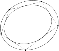
Fig. 6.2 Example of inner and outer ellipsoidal approximations of a pentagon in ${\mathbb{R}}^2$.

6.3.3 Polynomial curve-fitting

Consider a univariate polynomial of degree $n$,

$$f(t)=x_0+x_{1}t+x_2{t}^2+\cdots +x_n{t}^n.$$

Often we wish to fit such a polynomial to a given set of measurements or control points

$$\{(t_1,y_1),(t_2,y_2),\dots ,(t_m,y_m)\},$$

i.e., we wish to determine coefficients $x_i,i=0,\dots ,n$ such that

$$f(t_j)\approx y_j,j=1,\dots ,m.$$

To that end, define the Vandermonde matrix

$$\begin{array}{r}A=\left[\begin{array}{ccccc}1& t_1& t_1^2& \dots & t_1^n\\ 1& t_2& t_2^2& \dots & t_2^n\\ ⋮& ⋮& ⋮& & ⋮\\ 1& t_m& t_m^2& \dots & t_m^n\end{array}\right].\end{array}$$

We can then express the desired curve-fit compactly as

$$Ax\approx y,$$

i.e., as a linear expression in the coefficients $x$. When the degree of the polynomial equals the number measurements, $n=m$, the matrix $A$ is square and non-singular (provided there are no duplicate rows), so we can can solve

$$Ax=y$$

to find a polynomial that passes through all the control points $(t_i,y_i)$. Similarly, if $n>m$ there are infinitely many solutions satisfying the underdetermined system $Ax=y$. A typical choice in that case is the least-norm solution

$$x_{\ln }=\arg \underset{Ax=y}{min}\Vert x{\Vert }_2$$

which (assuming again there are no duplicate rows) equals

$$x_{\ln }=A^T(A{A}^T{)}^{-1}y.$$

On the other hand, if $n<m$ we generally cannot find a solution to the overdetermined system $Ax=y$, and we typically resort to a least-squares solution

$$x_{\mathrm{ls}}=\arg min\Vert Ax-y{\Vert }_2$$

which is given by the formula (see Sec. 8.5.1 (Linear regression and the normal equation))

$$x_{\mathrm{ls}}=(A^{T}A{)}^{-1}{A}^{T}y.$$

In the following we discuss how the semidefinite characterizations of nonnegative polynomials (see Sec. 6.2.6 (Nonnegative polynomials)) lead to more advanced and useful polynomial curve-fitting constraints.

• Nonnegativity. One possible constraint is nonnegativity on an interval,

  $$f(t):=x_0+x_{1}t+\cdots +x_n{t}^n\ge 0,\mathrm{\forall }t\in [a,b]$$

  with a semidefinite characterization embedded in $x\in K_{a,b}^n$, see (6.25).

• Monotonicity. We can ensure monotonicity of $f(t)$ by requiring that $f^{\prime }(t)\ge 0$ (or $f^{\prime }(t)\le 0$), i.e.,

  $$(x_1,2x_2,\dots ,n{x}_n)\in K_{a,b}^{n-1},$$

  or

  $$-(x_1,2x_2,\dots ,n{x}_n)\in K_{a,b}^{n-1},$$

  respectively.

• Convexity or concavity. Convexity (or concavity) of $f(t)$ corresponds to $f^{″}(t)\ge 0$ (or $f^{″}(t)\le 0$), i.e.,

  $$(2x_2,6x_3,\dots ,(n-1)n{x}_n)\in K_{a,b}^{n-2},$$

  or

  $$-(2x_2,6x_3,\dots ,(n-1)n{x}_n)\in K_{a,b}^{n-2},$$

  respectively.

As an example, we consider fitting a smooth polynomial

$$f_n(t)=x_0+x_{1}t+\cdots +x_n{t}^n$$

to the points $\{(-1,1),(0,0),(1,1)\}$, where smoothness is implied by bounding $|f_n^{\prime }(t)|$. More specifically, we wish to solve the problem

$$\begin{array}{r}\begin{array}{ll}\text{minimize}& z\\ \text{subject to}& |f_n^{\prime }(t)|\le z,\mathrm{\forall }t\in [-1,1]\\ & f_n(-1)=1,f_n(0)=0,f_n(1)=1,\end{array}\end{array}$$

or equivalently

$$\begin{array}{r}\begin{array}{ll}\text{minimize}& z\\ \text{subject to}& z-f_n^{\prime }(t)\ge 0,\mathrm{\forall }t\in [-1,1]\\ & f_n^{\prime }(t)-z\ge 0,\mathrm{\forall }t\in [-1,1]\\ & f_n(-1)=1,f_n(0)=0,f_n(1)=1.\end{array}\end{array}$$

Finally, we use the characterizations $K_{a,b}^n$ to get a conic problem

$$\begin{array}{r}\begin{array}{ll}\text{minimize}& z\\ \text{subject to}& (z-x_1,-2x_2,\dots ,-n{x}_n)\in K_{-1,1}^{n-1}\\ & (x_1-z,2x_2,\dots ,n{x}_n)\in K_{-1,1}^{n-1}\\ & f_n(-1)=1,f_n(0)=0,f_n(1)=1.\end{array}\end{array}$$

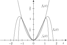
Fig. 6.3 Graph of univariate polynomials of degree 2, 4, and 8, respectively, passing through $\{(-1,1),(0,0),(1,1)\}$. The higher-degree polynomials are increasingly smoother on $[-1,1]$.

In Fig. 6.3 we show the graphs for the resulting polynomails of degree 2, 4 and 8, respectively. The second degree polynomial is uniquely determined by the three constraints $f_2(-1)=1$, $f_2(0)=0$, $f_2(1)=1$, i.e., $f_2(t)=t^2$. Also, we obviously have a lower bound on the largest derivative $\underset{t\in [-1,1]}{max}|f_n^{\prime }(t)|\ge 1$. The computed fourth degree polynomial is given by

$$f_4(t)=\frac{3}{2}{t}^2-\frac{1}{2}{t}^4$$

after rounding coefficients to rational numbers. Furthermore, the largest derivative is given by

$$f_4^{\prime }(1/\sqrt{2})=\sqrt{2},$$

and $f_4^{″}(t)<0$ on $(1/\sqrt{2},1]$ so, although not visibly clear, the polynomial is nonconvex on $[-1,1]$. In Fig. 6.4 we show the graphs of the corresponding polynomials where we added a convexity constraint $f_n^{″}(t)\ge 0$, i.e.,

$$(2x_2,6x_3,\dots ,(n-1)n{x}_n)\in K_{-1,1}^{n-2}.$$

In this case, we get

$$f_4(t)=\frac{6}{5}{t}^2-\frac{1}{5}{t}^4$$

and the largest derivative increases to $\frac{8}{5}$.

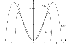
Fig. 6.4 Graph of univariate polynomials of degree $2,4,$ and $8$, respectively, passing through $\{(-1,1),(0,0),(1,1)\}$. The polynomials all have positive second derivative (i.e., they are convex) on $[-1,1]$ and the higher-degree polynomials are increasingly smoother on that interval.

6.3.4 Filter design problems

Filter design is an important application of optimization over trigonometric polynomials in signal processing. We consider a trigonometric polynomial

$$\begin{array}{r}\begin{array}{cl}H(\omega )& =x_0+2\mathrm{\Re }(\sum _{k=1}^n{x}_k{e}^{-j\omega k})\\ & =a_0+2\sum _{k=1}^n(a_k\cos (\omega k)+b_k\sin (\omega k))\end{array}\end{array}$$

where $a_k:=\mathrm{\Re }(x_k)$, $b_k:=\mathrm{\Im }(x_k)$. If the function $H(\omega )$ is nonnegative we call it a transfer function, and it describes how different harmonic components of a periodic discrete signal are attenuated when a filter with transfer function $H(\omega )$ is applied to the signal.

We often wish a transfer function where $H(\omega )\approx 1$ for $0\le \omega \le {\omega }_p$ and $H(\omega )\approx 0$ for ${\omega }_s\le \omega \le \pi$ for given constants ${\omega }_p,{\omega }_s$. One possible formulation for achieving this is

$$\begin{array}{r}\begin{array}{lcccccl}\text{minimize}& & & t& & & \\ \text{subject to}& 0& \le & H(\omega )& & & \mathrm{\forall }\omega \in [0,\pi ]\\ & 1-\delta & \le & H(\omega )& \le & 1+\delta & \mathrm{\forall }\omega \in [0,{\omega }_p]\\ & & & H(\omega )& \le & t& \mathrm{\forall }\omega \in [{\omega }_s,\pi ],\end{array}\end{array}$$

which corresponds to minimizing $H(w)$ on the interval $[{\omega }_s,\pi ]$ while allowing $H(w)$ to depart from unity by a small amount $\delta$ on the interval $[0,{\omega }_p]$. Using the results from Sec. 6.2.8 (Nonnegative trigonometric polynomials) (in particular (6.32), (6.33) and (6.34)), we can pose this as a conic optimization problem

(6.36)$$\begin{array}{r}\begin{array}{lrc}\text{minimize}& t& \\ \text{subject to}& x& \in & K_{0,\pi }^n,\\ & (x_0-(1-\delta ),x_{1:n})& \in & K_{0,{\omega }_p}^n,\\ & -(x_0-(1+\delta ),x_{1:n})& \in & K_{0,{\omega }_p}^n,\\ & -(x_0-t,x_{1:n})& \in & K_{{\omega }_s,\pi }^n,\end{array}\end{array}$$

which is a semidefinite optimization problem. In Fig. 6.5 we show $H(\omega )$ obtained by solving (6.36) for $n=10$, $\delta =0.05$, ${\omega }_p=\pi /4$ and ${\omega }_s={\omega }_p+\pi /8$.

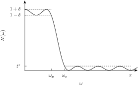
Fig. 6.5 Plot of lowpass filter transfer function.

6.3.5 Relaxations of binary optimization

Semidefinite optimization is also useful for computing bounds on difficult non-convex or combinatorial optimization problems. For example consider the binary linear optimization problem

(6.37)$$\begin{array}{r}\begin{array}{ll}\text{minimize}& c^{T}x\\ \text{subject to}& Ax=b,\\ & x\in \{0,1{\}}^n.\end{array}\end{array}$$

In general, problem (6.37) is a very difficult non-convex problem where we have to explore $2^n$ different objectives. Alternatively, we can use semidefinite optimization to get a lower bound on the optimal solution with polynomial complexity. We first note that

$$x_i\in \{0,1\}⟺x_i^2=x_i,$$

which is, in fact, equivalent to a rank constraint on a semidefinite variable,

$$X=x{x}^T,\mathbf{diag}(X)=x.$$

By relaxing the rank 1 constraint on $X$ we get a semidefinite relaxation of (6.37),

(6.38)$$\begin{array}{r}\begin{array}{ll}\text{minimize}& c^{T}x\\ \text{subject to}& Ax=b,\\ & \mathbf{diag}(X)=x,\\ & X⪰x{x}^T,\end{array}\end{array}$$

where we note that

$$\begin{array}{r}X⪰x{x}^T⟺\left[\begin{array}{cc}1& x^T\\ x& X\end{array}\right]⪰0.\end{array}$$

Since (6.38) is a semidefinite optimization problem, it can be solved very efficiently. Suppose $x^{\star }$ is an optimal solution for (6.37); then $(x^{\star },x^{\star }(x^{\star }{)}^T)$ is also feasible for (6.38), but the feasible set for (6.38) is larger than the feasible set for (6.37), so in general the optimal solution of (6.38) serves as a lower bound. However, if the optimal solution $X^{\star }$ of (6.38) has rank 1 we have found a solution to (6.37) also. The semidefinite relaxation can also be used in a branch-bound mixed-integer exact algorithm for (6.37).

We can tighten (or improve) the relaxation (6.38) by adding other constraints that cut away parts of the feasible set, without excluding rank 1 solutions. By tightening the relaxation, we reduce the gap between the optimal values of the original problem and the relaxation. For example, we can add the constraints

$$\begin{array}{r}\begin{array}{l}0\le X_{ij}\le 1,i=1,\dots ,n,j=1,\dots ,n,\\ X_{ii}\ge X_{ij},i=1,\dots ,n,j=1,\dots ,n,\end{array}\end{array}$$

and so on. This will usually have a dramatic impact on solution times and memory requirements. Already constraining a semidefinite matrix to be doubly nonnegative ($X_{ij}\ge 0$) introduces additional $n^2$ linear inequality constraints.

6.3.6 Relaxations of boolean optimization

Similarly to Sec. 6.3.5 (Relaxations of binary optimization) we can use semidefinite relaxations of boolean constraints $x\in \{-1,+1{\}}^n$. To that end, we note that

(6.39)$$x\in \{-1,+1{\}}^n⟺X=x{x}^T,\mathbf{diag}(X)=e,$$

with a semidefinite relaxation $X⪰x{x}^T$ of the rank-1 constraint.

As a (standard) example of a combinatorial problem with boolean constraints, we consider an undirected graph $G=(V,E)$ described by a set of vertices $V=\{v_1,\dots ,v_n\}$ and a set of edges $E=\{(v_i,v_j)\mid v_i,v_j\in V,i\ne j\}$, and we wish to find the cut of maximum capacity. A cut $C$ partitions the nodes $V$ into two disjoint sets $S$ and $T=V\setminus S$, and the cut-set $I$ is the set of edges with one node in $S$ and another in $T$, i.e.,

$$I=\{(u,v)\in E\mid u\in S,v\in T\}.$$

The capacity of a cut is then defined as the number of edges in the cut-set, $|I|$.

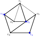
Fig. 6.6 Undirected graph. The cut $\{v_2,v_4,v_5\}$ has capacity 9 (thick edges).

To maximize the capacity of a cut we define the symmetric adjacency matrix $A\in {\mathcal{S}}^n$,

$$\begin{array}{r}[A{]}_{ij}=\{\begin{array}{ll}1,& (v_i,v_j)\in E,\\ 0,& \text{otherwise},\end{array}\end{array}$$

where $n=|V|$, and let

$$\begin{array}{r}{x}_i=\{\begin{array}{ll}+1,& v_i\in S,\\ -1,& v_i\notin S.\end{array}\end{array}$$

Suppose $v_i\in S$. Then $1-x_i{x}_j=0$ if $v_j\in S$ and $1-x_i{x}_j=2$ if $v_j\notin S$, so we get an expression for the capacity as

$$c(x)=\frac{1}{4}\sum _{ij}(1-x_i{x}_j)A_{ij}=\frac{1}{4}{e}^{T}Ae-\frac{1}{4}{x}^{T}Ax,$$

and discarding the constant term $e^{T}Ae$ gives us the MAX-CUT problem

(6.40)$$\begin{array}{r}\begin{array}{ll}\text{minimize}& x^{T}Ax\\ \text{subject to}& x\in \{-1,+1{\}}^n,\end{array}\end{array}$$

with a semidefinite relaxation

(6.41)$$\begin{array}{r}\begin{array}{ll}\text{minimize}& ⟨A,X⟩\\ \text{subject to}& \mathbf{diag}(X)=e,\\ & X⪰0.\end{array}\end{array}$$