7 Practical optimization

In this chapter we discuss various practical aspects of creating optimization models.

7.1 Conic reformulations

Many nonlinear constraint families were reformulated to conic form in previous chapters, and these examples are often sufficient to construct conic models for the optimization problems at hand. In case you do need to go beyond the cookbook examples, however, a few composition rules are worth knowing to guarantee correctness of your reformulation.

7.1.1 Perspective functions

The perspective of a function $f(x)$ is defined as $sf(x/s)$ on $s>0$. From any conic representation of $t\ge f(x)$ one can reach a representation of $t\ge sf(x/s)$ by exchanging all constants $k$ with their homogenized counterpart $ks$.

Example 7.1

In Sec. 5.2.6 (Log-sum-exp) it was shown that the logarithm of sum of exponentials

$$t\ge \log (e^{x_1}+\cdots +e^{x_n}),$$

can be modeled as:

$$\begin{array}{r}\begin{array}{rcl}\sum u_i& \le & 1,\\ (u_i,1,x_i-t)& \in & K_{\exp },i=1,\dots ,n.\end{array}\end{array}$$

It follows immediately that its perspective

$$t\ge s\log (e^{x_1/s}+\cdots +e^{x_n/s}),$$

can be modeled as:

$$\begin{array}{r}\begin{array}{rcl}\sum u_i& \le & s,\\ (u_i,s,x_i-t)& \in & K_{\exp },i=1,\dots ,n.\end{array}\end{array}$$

Proof

7.1

If $[t\ge f(x)]$ $\iff$ $[t\ge c(x,r)+c_0,A(x,r)+b\in K]$ for some linear functions $c$ and $A$, a cone $K$, and artificial variable $r$, then $[t\ge sf(x/s)]$ $\iff$ $[t\ge s(c(x/s,r)+c_0),A(x/s,r)+b\in K]$ $\iff$ $[t\ge c(x,\overline{r})+c_{0}s,A(x,\overline{r})+bs\in K]$, where $\overline{r}$ is taken as a new artificial variable in place of $rs$.

7.1.2 Composite functions

In representing composites $f(g(x))$, it is often helpful to move the inner function $g(x)$ to a separate constraint. That is, we would like $t\ge f(g(x))$ to be reformulated as $t\ge f(r)$ for a new variable $r$ constrained as $r=g(x)$. This reformulation works directly as stated if $g$ is affine; that is, $g(x)=a^{T}x+b$. Otherwise, one of two possible relaxations may be considered:

1. If $f$ is convex and $g$ is convex, then $t\ge f(r),r\ge g(x)$ is equivalent to $t\ge \{\begin{array}{ll}f(g(x))& \text{ if }g(x)\in {\mathcal{F}}^{+},\\ f_{min}& \text{ otherwise },\end{array}$

2. If $f$ is convex and $g$ is concave, then $t\ge f(r),r\le g(x)$ is equivalent to $t\ge \{\begin{array}{ll}f(g(x))& \text{ if }g(x)\in {\mathcal{F}}^{-},\\ f_{min}& \text{ otherwise },\end{array}$

where ${\mathcal{F}}^{+}$ (resp. ${\mathcal{F}}^{-}$) is the domain on which $f$ is nondecreasing (resp. nonincreasing), and $f_{min}$ is the minimum of $f$, if finite, and $-\mathrm{\infty }$ otherwise. Note that Relaxation 1 provides an exact representation if $g(x)\in {\mathcal{F}}^{+}$ for all $x$ in domain, and likewise for Relaxation 2 if $g(x)\in {\mathcal{F}}^{-}$ for all $x$ in domain.

Proof

7.2

Consider Relaxation 1. Intuitively, if $r\in {\mathcal{F}}^{+}$, you can expect clever solvers to drive $r$ towards $-\mathrm{\infty }$ in attempt to relax $t\ge f(r)$, and this push continues until $r\ge g(x)$ becomes active or else — in case $g(x)\notin {\mathcal{F}}^{+}$ — until $f_{min}$ is reached. On the other hand, if $r\in {\mathcal{F}}^{-}$ (and thus $r\ge g(x)\in {\mathcal{F}}^{-}$) then solvers will drive $r$ towards $+\mathrm{\infty }$ until $f_{min}$ is reached.

Example 7.2

Here are some simple substitutions.

• The inequality $t\ge \exp (g(x))$ can be rewritten as $t\ge \exp (r)$ and $r\ge g(x)$ for all convex functions $g(x)$. This is because $f(r)=\exp (r)$ is nondecreasing everywhere.

• The inequality $2st\ge g(x{)}^2$ can be rewritten as $2st\ge r^2$ and $r\ge g(x)$ for all nonnegative convex functions $g(x)$. This is because $f(r)=r^2$ is nondecreasing on $r\ge 0$.

• The nonconvex inequality $t\ge (x^2-1{)}^2$ can be relaxed as $t\ge r^2$ and $r\ge x^2-1$. This relaxation is exact on $x^2-1\ge 0$ where $f(r)=r^2$ is nondecreasing, i.e., on the disjoint domain $|x|\ge 1$. On the domain $|x|\le 1$ it represents the strongest possible convex cut given by $t\ge f_{min}=0$.

Example 7.3

Some amount of work is generally required to find the correct reformulation of a nested nonlinear constraint. For instance, suppose that for $x,y,z\ge 0$ with $xyz>1$ we want to write

$$t\ge \frac{1}{xyz-1}.$$

A natural first attempt is:

$$t\ge \frac{1}{r},r\le xyz-1,$$

which corresponds to Relaxation 2 with $f(r)=1/r$ and $g(x,y,z)=xyz-1>0$. The function $f$ is indeed convex and nonincreasing on all of $g(x,y,z)$, and the inequality $tr\ge 1$ is moreover representable with a rotated quadratic cone. Unfortunately $g$ is not concave. We know that a monomial like $xyz$ appears in connection with the power cone, but that requires a homogeneous constraint such as $xyz\ge u^3$. This gives us an idea to try

$$t\ge \frac{1}{r^3},r^3\le xyz-1,$$

which is $f(r)=1/r^3$ and $g(x,y,z)=(xyz-1{)}^{1/3}>0$. This provides the right balance: all conditions for validity and exactness of Relaxation 2 are satisfied. Introducing another variable $u$ we get the following model:

$$t{r}^3\ge 1,xyz\ge u^3,u\ge (r^3+1^3{)}^{1/3},$$

We refer to Sec. 4 (The power cones) to verify that all the constraints above are representable using power cones. We leave it as an exercise to find other conic representations, based on other transformations of the original inequality.

7.1.3 Convex univariate piecewise-defined functions

Consider a univariate function with $k$ pieces:

$$\begin{array}{r}f(x)=\{\begin{array}{ll}{f}_1(x)& \text{ if }x\le {\alpha }_1,\\ f_i(x)& \text{ if }{\alpha }_{i-1}\le x\le {\alpha }_i,\text{ for }i=2,\dots ,k-1,\\ f_k(x)& \text{ if }{\alpha }_{k-1}\le x,\end{array}\end{array}$$

Suppose $f(x)$ is convex (in particular each piece is convex by itself) and $f_i({\alpha }_i)=f_{i+1}({\alpha }_i)$. In representing the epigraph $t\ge f(x)$ it is helpful to proceed via the equivalent representation:

$$\begin{array}{r}\begin{array}{l}t=\sum _{i=1}^k{t}_i-\sum _{i=1}^{k-1}{f}_i({\alpha }_i),\\ x=\sum _{i=1}^k{x}_i-\sum _{i=1}^{k-1}{\alpha }_i,\\ t_i\ge f_i(x_i)\text{ for }i=1,\dots ,k,\\ x_1\le {\alpha }_1,{\alpha }_{i-1}\le x_i\le {\alpha }_i\text{ for }i=2,\dots ,k-1,{\alpha }_{k-1}\le x_k.\end{array}\end{array}$$

Proof

7.3

In the special case when $k=2$ and ${\alpha }_1=f_1({\alpha }_1)=f_2({\alpha }_1)=0$ the epigraph of $f$ is equal to the Minkowski sum $\{(t_1+t_2,x_1+x_2):t_i\ge f_i(x_i)\}$. In general the epigraph over two consecutive pieces is obtained by shifting them to $(0,0)$, computing the Minkowski sum and shifting back. Finally more than two pieces can be joined by continuing this argument by induction.

As the reformulation grows in size with the number of pieces, it is preferable to keep this number low. Trivially, if $f_i(x)=f_{i+1}(x)$, these two pieces can be merged. Substituting $f_i(x)$ and $f_{i+1}(x)$ for $max(f_i(x),f_{i+1}(x))$ is sometimes an invariant change to facilitate this merge. For instance, it always works for affine functions $f_i(x)$ and $f_{i+1}(x)$. Finally, if $f(x)$ is symmetric around some point $\alpha$, we can represent its epigraph via a piecewise function, with only half the number of pieces, defined in terms of a new variable $z=|x-\alpha |+\alpha$.

Example 7.4 Huber loss function

The Huber loss function

$$\begin{array}{r}f(x)=\{\begin{array}{ll}-2x-1& \text{ if }x\le -1,\\ x^2& \text{ if }-1\le x\le 1,\\ 2x-1& \text{ if }1\le x,\end{array}\end{array}$$

is convex and its epigraph $t\ge f(x)$ has an equivalent representation

$$\begin{array}{r}\begin{array}{l}t\ge t_1+t_2+t_3-2,\\ x=x_1+x_2+x_3,\\ t_1=-2x_1-1,t_2\ge x_2^2,t_3=2x_3-1,\\ x_1\le -1,-1\le x_2\le 1,1\le x_3,\end{array}\end{array}$$

where $t_2\ge x_2^2$ is representable by a rotated quadratic cone. No two pieces of $f(x)$ can be merged to reduce the size of this formulation, but the loss function does satisfy a simple symmetry; namely $f(x)=f(-x)$. We can thus represent its epigraph by $t\ge \hat{f}(z)$ and $z\ge |x|$, where

$$\begin{array}{r}\hat{f}(z)=\{\begin{array}{ll}{z}^2& \text{ if }z\le 1,\\ 2z-1& \text{ if }1\le z.\end{array}\end{array}$$

In this particular example, however, unless the absolute value $z$ from $z\ge |x|$ is used elsewhere, the cost of introducing it does not outweigh the savings achieved by going from three pieces in $x$ to two pieces in $z$.

7.2 Avoiding ill-posed problems

For a well-posed continuous problem a small change in the input data should induce a small change of the optimal solution. A problem is ill-posed if small perturbations of the problem data result in arbitrarily large perturbations of the solution, or even change the feasibility status of the problem. In such cases small rounding errors, or solving the problem on a different computer can result in different or wrong solutions.

In fact, from an algorithmic point of view, even computing a wrong solution is numerically difficult for ill-posed problems. A rigorous definition of the degree of ill-posedness is possible by defining a condition number. This is an attractive, but not very practical metric, as its evaluation requires solving several auxiliary optimization problems. Therefore we only make the modest recommendations to avoid problems

• that are nearly infeasible,

• with constraints that are linearly dependent, or nearly linearly dependent.

Example 7.5 Near linear dependencies

To give some idea about the perils of near linear dependence, consider this pair of optimization problems:

$$\begin{array}{r}\begin{array}{lrcl}\text{maximize}& x& & \\ \text{subject to }& 2x-y& \ge & -1,\\ & 2.0001x-y& \le & 0,\end{array}\end{array}$$

and

$$\begin{array}{r}\begin{array}{lrcl}\text{maximize}& x& & \\ \text{subject to }& 2x-y& \ge & -1,\\ & 1.9999x-y& \le & 0.\end{array}\end{array}$$

The first problem has a unique optimal solution $(x,y)=({10}^4,2\cdot {10}^4+1)$, while the second problem is unbounded. This is caused by the fact that the hyperplanes (here: straight lines) defining the constraints in each problem are almost parallel. Moreover, we can consider another modification:

$$\begin{array}{r}\begin{array}{lrcl}\text{maximize}& x& & \\ \text{subject to }& 2x-y& \ge & -1,\\ & 2.001x-y& \le & 0,\end{array}\end{array}$$

with optimal solution $(x,y)=({10}^3,2\cdot {10}^3+1)$, which shows how a small perturbation of the coefficients induces a large change of the solution.

Typical examples of problems with nearly linearly dependent constraints are discretizations of continuous processes, where the constraints invariably become more correlated as we make the discretization finer; as such there may be nothing wrong with the discretization or problem formulation, but we should expect numerical difficulties for sufficiently fine discretizations.

One should also be careful not to specify problems whose optimal value is only achieved in the limit. A trivial example is

$$\text{minimize}{e}^x,x\in \mathbb{R}.$$

The infimum value 0 is not attained for any finite $x$, which can lead to unspecified behaviour of the solver. More examples of ill-posed conic problems are discussed in Fig. 7.1 and Sec. 8 (Duality in conic optimization). In particular, Fig. 7.1 depicts some troublesome problems in two dimensions. In (a) minimizing $y\ge 1/x$ on the nonnegative orthant is unattained approaching zero for $x\to \mathrm{\infty }$. In (b) the only feasible point is $(0,0)$, but objectives maximizing $x$ are not blocked by the purely vertical normal vectors of active constraints at this point, falsely suggesting local progress could be made. In (c) the intersection of the two subsets is empty, but the distance between them is zero. Finally in (d) minimizing $x$ on $y\ge x^2$ is unbounded at minus infinity for $y\to \mathrm{\infty }$, but there is no improving ray to follow. Although seemingly unrelated, the four cases are actually primal-dual pairs; (a) with (b) and (c) with (d). In fact, the missing normal vector property in (b)—desired to certify optimality—can be attributed to (a) not attaining the best among objective values at distance zero to feasibility, and the missing positive distance property in (c)—desired to certify infeasibility—is because (d) has no improving ray.

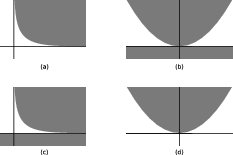
Fig. 7.1 Geometric representations of some ill-posed situations.

7.3 Scaling

Another difficulty encountered in practice involves models that are badly scaled. Loosely speaking, we consider a model to be badly scaled if

• variables are measured on very different scales,

• constraints or bounds are measured on very different scales.

For example if one variable $x_1$ has units of molecules and another variable $x_2$ measures temperature, we might expect an objective function such as

$$x_1+{10}^{12}{x}_2$$

and in finite precision the second term dominates the objective and renders the contribution from $x_1$ insignificant and unreliable.

A similar situation (from a numerical point of view) is encountered when using penalization or big-$M$ strategies. Assume we have a standard linear optimization problem (2.12) with the additional constraint that $x_1=0$. We may eliminate $x_1$ completely from the model, or we might add an additional constraint, but suppose we choose to formulate a penalized problem instead

$$\begin{array}{r}\begin{array}{ll}\text{minimize}& c^{T}x+{10}^{12}{x}_1\\ \text{subject to}& Ax=b,\\ & x\ge 0,\end{array}\end{array}$$

reasoning that the large penalty term will force $x_1=0$. However, if $\Vert c\Vert$ is small we have the exact same problem, namely that in finite precision the penalty term will completely dominate the objective and render the contribution $c^{T}x$ insignificant or unreliable. Therefore, the penalty term should be chosen carefully.

Example 7.6 Risk-return tradeoff

Suppose we want to solve an efficient frontier variant of the optimal portfolio problem from Sec. 3.3.3 (Markowitz portfolio optimization) with an objective of the form

$$\text{maximize}{\mu }^{T}x-\frac{1}{2}\gamma x^T\mathrm{\Sigma }x$$

where the parameter $\gamma$ controls the tradeoff between return and risk. The user might choose a very small $\gamma$ to discount the risk term. This, however, may lead to numerical issues caused by a very large solution. To see why, consider a simple one-dimensional, unconstrained analogue:

$$\text{maximize}x-\frac{1}{2}\gamma x^2,x\in \mathbb{R}$$

and note that the maximum is attained for $x=1/\gamma$, which may be very large.

Example 7.7 Explicit redundant bounds

Consider again the problem (2.12), but with additional (redundant) constraints $x_i\le \gamma$. This is a common approach for some optimization practitioners. The problem we solve is then

$$\begin{array}{r}\begin{array}{ll}\text{minimize}& c^{T}x\\ \text{subject to}& Ax=b,\\ & x\ge 0,\\ & x\le \gamma e,\end{array}\end{array}$$

with a dual problem

$$\begin{array}{r}\begin{array}{ll}\text{maximize}& b^{T}y-\gamma e^{T}z\\ \text{subject to}& A^{T}y+s-z=c,\\ & s,z\ge 0.\end{array}\end{array}$$

Suppose we do not know a-priori an upper bound on $\Vert x{\Vert }_{\mathrm{\infty }}$, so we choose a very large $\gamma ={10}^{12}$ reasoning that this will not change the optimal solution. Note that the large variable bound becomes a penalty term in the dual problem; in finite precision such a large bound will effectively destroy accuracy of the solution.

Example 7.8 Big-M

Suppose we have a mixed integer model which involves a big-M constraint (see Sec. 9 (Mixed integer optimization)), for instance

$$a^{T}x\le b+M(1-z)$$

as in Sec. 9.1.3 (Indicator constraints). The constant $M$ must be big enough to guarantee that the constraint becomes redundant when $z=0$, or we risk shrinking the feasible set, perhaps to the point of creating an infeasible model. On the other hand, the user might set $M$ to a huge, safe value, say $M={10}^{12}$. While this is mathematically correct, it will lead to a model with poorer linear relaxations and most likely increase solution time (sometimes dramatically). It is therefore very important to put some effort into estimating a reasonable value of $M$ which is safe, but not too big.

7.4 The huge and the tiny

Some types of problems and constraints are especially prone to behave badly with very large or very small numbers. We discuss such examples briefly in this section.

Sum of squares

The sum of squares $x_1^2+\cdots +x_n^2$ can be bounded above using the rotated quadratic cone:

$$t\ge x_1^2+\cdots +x_n^2⟺(\frac{1}{2},t,x)\in {\mathcal{Q}}_{\mathit{r}}^n,$$

but in most cases it is better to bound the square root with a quadratic cone:

$$t^{\prime }\ge \sqrt{x_1^2+\cdots +x_n^2}⟺(t^{\prime },x)\in {\mathcal{Q}}^n.$$

The latter has slightly better numerical properties: $t^{\prime }$ is roughly comparable with $x$ and is measured on the same scale, while $t$ grows as the square of $x$ which will sooner lead to numerical instabilities.

Exponential cone

Using the function $e^x$ for $x\le -30$ or $x\ge 30$ would be rather questionable if $e^x$ is supposed to represent any realistic value. Note that $e^{30}\approx {10}^{13}$ and that $e^{30.0000001}-e^{30}\approx {10}^6$, so a tiny perturbation of the exponent produces a huge change of the result. Ideally, $x$ should have a single-digit absolute value. For similar reasons, it is even more important to have well-scaled data. For instance, in floating point arithmetic we have the “equality”

$$e^{20}+e^{-20}=e^{20}$$

since the smaller summand disappears in comparison to the other one, ${10}^{17}$ times bigger.

For the same reason it is advised to replace explicit inequalities involving $\exp (x)$ with log-sum-exp variants (see Sec. 5.2.6 (Log-sum-exp)). For example, suppose we have a constraint such as

$$t\ge e^{x_1}+e^{x_2}+e^{x_3}.$$

Then after a substitution $t=e^{t^{\prime }}$ we have

$$1\ge e^{x_1-t^{\prime }}+e^{x_2-t^{\prime }}+e^{x_3-t^{\prime }}$$

which has the advantage that $t^{\prime }$ is of the same order of magnitude as $x_i$, and that the exponents $x_i-t^{\prime }$ are likely to have much smaller absolute values than simply $x_i$.

Power cone

The power cone is not reliable when one of the exponents is very small. For example, consider the function $f(x)=x^{0.01}$, which behaves almost like the indicator function of $x>0$ in the sense that

$$f(0)=0,\text{and}f(x)>0.5\text{for}x>{10}^{-30}.$$

Now suppose $x={10}^{-20}$. Is the constraint $f(x)>0.5$ satisfied? In principle yes, but in practice $x$ could have been obtained as a solution to an optimization problem and it may in fact represent $0$ up to numerical error. The function $f(x)$ is sensitive to changes in $x$ well below standard numerical accuracy. The point $x=0$ does not satisfy $f(x)>0.5$ but it is only ${10}^{-30}$ from doing so.

7.5 Semidefinite variables

Special care should be given to models involving semidefinite matrix variables (see Sec. 6 (Semidefinite optimization)), otherwise it is easy to produce an unnecessarily inefficient model. The general rule of thumb is:

• having many small matrix variables is more efficient than one big matrix variable,

• efficiency drops with growing number of semidefinite terms involved in linear constraints. This can have much bigger impact on the solution time than increasing the dimension of the semidefinite variable.

Let us consider a few examples.

Block matrices

Given two matrix variables $X,Y⪰0$ do not assemble them in a block matrix and write the constraints as

$$\begin{array}{r}\left[\begin{array}{cc}X& 0\\ 0& Y\end{array}\right]⪰0.\end{array}$$

This increases the dimension of the problem and, even worse, introduces unnecessary constraints for a large portion of entries of the block matrix.

Schur complement

Suppose we want to model a relaxation of a rank-one constraint:

$$\begin{array}{r}\left[\begin{array}{cc}X& x\\ x^T& 1\end{array}\right]⪰0.\end{array}$$

where $x\in {\mathbb{R}}^n$ and $X\in {\mathcal{S}}_{+}^n$. The correct way to do this is to set up a matrix variable $Y\in {\mathcal{S}}_{+}^{n+1}$ with only a linear number of constraints:

$$\begin{array}{r}\begin{array}{ll}{Y}_{i,n+1}=x_i,& i=1,\dots ,n\\ Y_{n+1,n+1}=1,& \\ Y⪰0,& \end{array}\end{array}$$

and use the upper-left $n\times n$ part of $Y$ as the original $X$. Going the other way around, i.e. starting with a variable $X$ and aligning it with the corner of another, bigger semidefinite matrix $Y$ introduces $n(n+1)/2$ equality constraints and will quickly have formidable solution times.

Sparse LMIs

Suppose we want to model a problem with a sparse linear matrix inequality (see Sec. 6.2.1 (Linear matrix inequalities)) such as:

$$\begin{array}{r}\begin{array}{ll}\text{minimize}& c^{T}x\\ \text{subject to}& A_0+\sum _{i=1}^k{A}_i{x}_i⪰0,\end{array}\end{array}$$

where $x\in {\mathbb{R}}^k$ and $A_i$ are symmetric $n\times n$ matrices. The representation of this problem in primal form is:

$$\begin{array}{r}\begin{array}{ll}\text{minimize}& c^{T}x\\ \text{subject to}& A_0+\sum _{i=1}^k{A}_i{x}_i=X,\\ & X⪰0,\end{array}\end{array}$$

and the linear constraint requires a full set of $n(n+1)/2$ equalities, many of which are just $X_{k,l}=0$, regardless of the sparsity of $A_i$. However the dual problem (see Sec. 8.6 (Semidefinite duality and LMIs)) is:

$$\begin{array}{r}\begin{array}{ll}\text{maximize}& -⟨A_0,Z⟩\\ \text{subject to}& ⟨A_i,Z⟩=c_i,i=1,\dots ,k,\\ & Z⪰0,\end{array}\end{array}$$

and the number of nonzeros in linear constraints is just joint number of nonzeros in $A_i$. It means that large, sparse LMIs should almost always be dualized and entered in that form for efficiency reasons.

7.6 The quality of a solution

In this section we will discuss how to validate an obtained solution. Assume we have a conic model with continuous variables only and that the optimization software has reported an optimal primal and dual solution. Given such a solution, we might ask how to verify that it is indeed feasible and optimal.

To that end, consider a simple model

(7.1)$$\begin{array}{r}\begin{array}{lrc}\text{minimize}& -x_2& \\ \text{subject to}& x_1+x_2& \le & 3,\\ & x_2^2& \le & 2,\\ & x_1,x_2& \ge & 0,\end{array}\end{array}$$

where a solver might approximate the solution as

$$x_1=0.0000000000000000\text{ and }{x}_2=1.4142135623730951$$

and therefore the approximate optimal objective value is

$$-1.4142135623730951.$$

The true objective value is $-\sqrt{2}$, so the approximate objective value is wrong by the amount

$$1.4142135623730951-\sqrt{2}\approx {10}^{-16}.$$

Most likely this difference is irrelevant for all practical purposes. Nevertheless, in general a solution obtained using floating point arithmetic is only an approximation. Most (if not all) commercial optimization software uses double precision floating point arithmetic, implying that about 16 digits are correct in the computations performed internally by the software. This also means that irrational numbers such as $\sqrt{2}$ and $\pi$ can only be stored accurately within 16 digits.

Verifying feasibility

A good practice after solving an optimization problem is to evaluate the reported solution. At the very least this process should be carried out during the initial phase of building a model, or if the reported solution is unexpected in some way. The first step in that process is to check that the solution is feasible; in case of the small example (7.1) this amounts to checking that:

$$\begin{array}{r}\begin{array}{rcrcl}{x}_1+x_2& =& 0.0000000000000000+1.4142135623730951& \le & 3,\\ x_2^2& =& 2.0000000000000004& \le & 2,(?)\\ x_1& =& 0.0000000000000000& \ge & 0,\\ x_2& =& 1.4142135623730951& \ge & 0,\end{array}\end{array}$$

which demonstrates that one constraint is slightly violated due to computations in finite precision. It is up to the user to assess the significance of a specific violation; for example a violation of one unit in

$$x_1+x_2\le 1$$

may or may not be more significant than a violation of one unit in

$$x_1+x_2\le {10}^9.$$

The right-hand side of ${10}^9$ may itself be the result of a computation in finite precision, and may only be known with, say 3 digits of accuracy. Therefore, a violation of 1 unit is not significant since the true right-hand side could just as well be $1.001\cdot {10}^9$. Certainly a violation of $4\cdot {10}^{-16}$ as in our example is within the numerical tolerance for zero and we would accept the solution as feasible. In practice it would be standard to see violations of order ${10}^{-8}$.

Verifying optimality

Another question is how to verify that a feasible approximate solution is actually optimal, which is answered by duality theory, which is discussed in Sec. 2.4 (Duality in linear optimization) for linear problems and in Sec. 8 (Duality in conic optimization) in full generality. Following Sec. 8 (Duality in conic optimization) we can derive an equivalent version of the dual problem as:

$$\begin{array}{r}\begin{array}{lrcl}\text{maximize}& -3y_1-y_2-y_3& & \\ \text{subject to}& 2y_2{y}_3& \ge & (y_1+1{)}^2,\\ & y_1& \ge & 0.\end{array}\end{array}$$

This problem has a feasible point $(y_1,y_2,y_3)=(0,1/\sqrt{2},1/\sqrt{2})$ with objective value $-\sqrt{2}$, matching the objective value of the primal problem. By duality theory this proves that both the primal and dual solutions are optimal. Again, in finite precision the dual objective value may be reported as, for example

$$-1.4142135623730950$$

leading to a duality gap of about ${10}^{-16}$ between the approximate primal and dual objective values. It is up to the user to assess the significance of any duality gap and accept or reject the solution as sufficiently good approximation of the optimal value.

7.7 Distance to a cone

The violation of a linear constraint $a^{T}x\le b$ under a given solution $x^{\ast }$ is obviously

$$max(0,a^T{x}^{\ast }-b).$$

It is less obvious how to assess violations of conic constraints. To this end suppose we have a convex cone $K$. The (Euclidean) projection of a point $x$ onto $K$ is defined as the solution of the problem

(7.2)$$\begin{array}{r}\begin{array}{ll}\text{minimize}& \Vert p-x{\Vert }_2\\ \text{subject to}& p\in K.\end{array}\end{array}$$

We denote the projection by ${\mathrm{proj}}_K(x)$. The distance of $x$ to $K$

$$\mathrm{dist}(x,K)=\Vert x-{\mathrm{proj}}_K(x){\Vert }_2,$$

i.e. the objective value of (7.2), measures the violation of a conic constraint involving $K$. Obviously

$$\mathrm{dist}(x,K)=0⟺x\in K.$$

This distance measure is attractive because it depends only on the set $K$ and not on any particular representation of $K$ using (in)equalities.

Example 7.9 Surprisingly small distance

Let $K={\mathcal{P}}_3^{0.1,0.9}$ be the power cone defined by the inequality $x^{0.1}{y}^{0.9}\ge |z|$. The point

$$x^{\ast }=(x,y,z)=(0,10000,500)$$

is clearly not in the cone, in fact $x^{0.1}{y}^{0.9}=0$ while $|z|=500$, so the violation of the conic inequality is seemingly large. However, the point

$$p=({10}^{-8},10000,500)$$

belongs to ${\mathcal{P}}_3^{0.1,0.9}$ (since $({10}^{-8}{)}^{0.1}\cdot {10000}^{0.9}\approx 630$), hence

$$\mathrm{dist}(x^{\ast },{\mathcal{P}}_3^{0.1,0.9})\le \Vert x^{\ast }-p{\Vert }_2={10}^{-8}.$$

Therefore the distance of $x^{\ast }$ to the cone is actually very small.

Distance to certain cones

For some basic cone types the projection problem (7.2) can be solved analytically. Denoting $[x{]}_{+}=max(0,x)$ we have that:

• For $x\in \mathbb{R}$ the projection onto the nonnegative half-line is ${\mathrm{proj}}_{{\mathbb{R}}_{+}}(x)=[x{]}_{+}$.

• For $(t,x)\in \mathbb{R}\times {\mathbb{R}}^{n-1}$ the projection onto the quadratic cone is

  $$\begin{array}{r}{\mathrm{proj}}_{{\mathcal{Q}}^n}(t,x)=\{\begin{array}{ll}(t,x)& \text{if}t\ge \Vert x{\Vert }_2,\\ \frac{1}{2}(\frac{t}{\Vert x{\Vert }_2}+1)(\Vert x{\Vert }_2,x)& \text{if}-\Vert x{\Vert }_2<t<\Vert x{\Vert }_2,\\ 0& \text{if}t\le -\Vert x{\Vert }_2.\end{array}\end{array}$$

• For $X=\sum _{i=1}^n{\lambda }_i{q}_i{q}_i^T$ the projection onto the semidefinite cone is

  $${\mathrm{proj}}_{{\mathcal{S}}_{+}^n}(X)=\sum _{i=1}^n[{\lambda }_i{]}_{+}{q}_i{q}_i^T.$$