2 Linear optimization

In this chapter we discuss various aspects of linear optimization. We first introduce the basic concepts of linear optimization and discuss the underlying geometric interpretations. We then give examples of the most frequently used reformulations or modeling tricks used in linear optimization, and finally we discuss duality and infeasibility theory in some detail.

2.1 Introduction

2.1.1 Basic notions

The most basic type of optimization is linear optimization. In linear optimization we minimize a linear function given a set of linear constraints. For example, we may wish to minimize a linear function

$$x_1+2x_2-x_3$$

under the constraints that

$$x_1+x_2+x_3=1,x_1,x_2,x_3\ge 0.$$

The function we minimize is often called the objective function; in this case we have a linear objective function. The constraints are also linear and consist of both linear equalities and inequalities. We typically use more compact notation

(2.1)$$\begin{array}{r}\begin{array}{ll}\text{minimize}& x_1+2x_2-x_3\\ \text{subject to}& x_1+x_2+x_3=1,\\ & x_1,x_2,x_3\ge 0,\end{array}\end{array}$$

and we call (2.1) a linear optimization problem. The domain where all constraints are satisfied is called the feasible set; the feasible set for (2.1) is shown in Fig. 2.1.

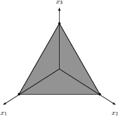
Fig. 2.1 Feasible set for $x_1+x_2+x_3=1$ and $x_1,x_2,x_3\ge 0.$

For this simple problem we see by inspection that the optimal value of the problem is $-1$ obtained by the optimal solution

$$(x_1^{\star },x_2^{\star },x_3^{\star })=(0,0,1).$$

Linear optimization problems are typically formulated using matrix notation. The standard form of a linear minimization problem is:

(2.2)$$\begin{array}{r}\begin{array}{ll}\text{minimize}& c^{T}x\\ \text{subject to}& Ax=b,\\ & x\ge 0.\end{array}\end{array}$$

For example, we can pose (2.1) in this form with

$$\begin{array}{r}x=\left[\begin{array}{c}{x}_1\\ x_2\\ x_3\end{array}\right],c=\left[\begin{array}{c}1\\ 2\\ -1\end{array}\right],A=\left[\begin{array}{ccc}1& 1& 1\end{array}\right].\end{array}$$

There are many other formulations for linear optimization problems; we can have different types of constraints,

$$Ax=b,Ax\ge b,Ax\le b,l^c\le Ax\le u^c,$$

and different bounds on the variables

$$l^x\le x\le u^x$$

or we may have no bounds on some $x_i$, in which case we say that $x_i$ is a free variable. All these formulations are equivalent in the sense that by simple linear transformations and introduction of auxiliary variables they represent the same set of problems. The important feature is that the objective function and the constraints are all linear in $x$.

2.1.2 Geometry of linear optimization

A hyperplane is a subset of ${\mathbb{R}}^n$ defined as $\{x\mid a^T(x-x_0)=0\}$ or equivalently $\{x\mid a^{T}x=\gamma \}$ with $a^T{x}_0=\gamma$, see Fig. 2.2.

Fig. 2.2 The dashed line illustrates a hyperplane $\{x\mid a^{T}x=\gamma \}$.

Thus a linear constraint

$$Ax=b$$

with $A\in {\mathbb{R}}^{m\times n}$ represents an intersection of $m$ hyperplanes.

Next, consider a point $x$ above the hyperplane in Fig. 2.3. Since $x-x_0$ forms an acute angle with $a$ we have that $a^T(x-x_0)\ge 0$, or $a^{T}x\ge \gamma$. The set $\{x\mid a^{T}x\ge \gamma \}$ is called a halfspace. Similarly the set $\{x\mid a^{T}x\le \gamma \}$ forms another halfspace; in Fig. 2.3 it corresponds to the area below the dashed line.

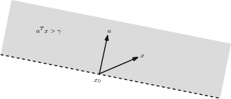
Fig. 2.3 The grey area is the halfspace $\{x\mid a^{T}x\ge \gamma \}$.

A set of linear inequalities

$$Ax\le b$$

corresponds to an intersection of halfspaces and forms a polyhedron, see Fig. 2.4.

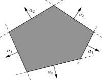
Fig. 2.4 A polyhedron formed as an intersection of halfspaces.

The polyhedral description of the feasible set gives us a very intuitive interpretation of linear optimization, which is illustrated in Fig. 2.5. The dashed lines are normal to the objective $c=(-1,1)$, and to minimize $c^{T}x$ we move as far as possible in the opposite direction of $c$, to the furthest position where a dashed line intersect the polyhedron; an optimal solution is therefore always either a vertex of the polyhedron, or an entire facet of the polyhedron may be optimal.

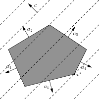
Fig. 2.5 Geometric interpretation of linear optimization. The optimal solution $x^{\star }$ is at a point where the normals to $c$ (the dashed lines) intersect the polyhedron.

The polyhedron shown in the figure is nonempty and bounded, but this is not always the case for polyhedra arising from linear inequalities in optimization problems. In such cases the optimization problem may be infeasible or unbounded, which we will discuss in detail in Sec. 2.3 (Infeasibility in linear optimization).

2.2 Linear modeling

In this section we present useful reformulation techniques and standard tricks which allow constructing more complicated models using linear optimization. It is also a guide through the types of constraints which can be expressed using linear (in)equalities.

2.2.1 Maximum

The inequality $t\ge max\{x_1,\dots ,x_n\}$ is equivalent to a simultaneous sequence of $n$ inequalities

$$t\ge x_i,i=1,\dots ,n$$

and similarly $t\le min\{x_1,\dots ,x_n\}$ is the same as

$$t\le x_i,i=1,\dots ,n.$$

Of course the same reformulation applies if each $x_i$ is not a single variable but a linear expression. In particular, we can consider convex piecewise-linear functions $f:{\mathbb{R}}^n\mapsto \mathbb{R}$ defined as the maximum of affine functions (see Fig. 2.6):

$$f(x):=\underset{i=1,\dots ,m}{max}\{a_i^{T}x+b_i\}$$

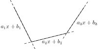
Fig. 2.6 A convex piecewise-linear function (solid lines) of a single variable $x$. The function is defined as the maximum of 3 affine functions.

The epigraph $f(x)\le t$ (see Sec. 12 (Notation and definitions)) has an equivalent formulation with $m$ inequalities:

$$a_i^{T}x+b_i\le t,i=1,\dots ,m.$$

Piecewise-linear functions have many uses linear in optimization; either we have a convex piecewise-linear formulation from the onset, or we may approximate a more complicated (nonlinear) problem using piecewise-linear approximations, although with modern nonlinear optimization software it is becoming both easier and more efficient to directly formulate and solve nonlinear problems without piecewise-linear approximations.

2.2.2 Absolute value

The absolute value of a scalar variable, $|x|:=max\{x,-x\}$, is a special case of Sec. 2.2.1 (Maximum). To model the epigraph

$$|x|\le t,$$

we can thus use two inequalities

$$-t\le x\le t.$$

2.2.3 The ${\ell }_1$ norm

All norms are convex functions, but the ${\ell }_1$ and ${\ell }_{\mathrm{\infty }}$ norms are of particular interest for linear optimization. The ${\ell }_1$ norm of vector $x\in {\mathbb{R}}^n$ is defined as

$$\Vert x{\Vert }_1:=|x_1|+|x_2|+\cdots +|x_n|.$$

To model the epigraph

(2.3)$$\Vert x{\Vert }_1\le t,$$

we introduce the following system

(2.4)$$|x_i|\le z_i,i=1,\dots ,n,\sum _{i=1}^n{z}_i=t,$$

with additional (auxiliary) variable $z\in {\mathbb{R}}^n$. Clearly (2.3) and (2.4) are equivalent, in the sense that they have the same projection onto the space of $x$ and $t$ variables. Therefore, we can model (2.3) using linear (in)equalities

(2.5)$$-z_i\le x_i\le z_i,\sum _{i=1}^n{z}_i=t,$$

with auxiliary variables $z$. Similarly, we can describe the epigraph of the norm of an affine function of $x$,

$$\Vert Ax-b{\Vert }_1\le t$$

as

$$-z_i\le a_i^{T}x-b_i\le z_i,\sum _{i=1}^n{z}_i=t,$$

where $a_i$ is the $i-$th row of $A$ (taken as a column-vector).

Example 2.1 Basis pursuit

The ${\ell }_1$ norm is overwhelmingly popular as a convex approximation of the cardinality (i.e., number on nonzero elements) of a vector $x$. For example, suppose we are given an underdetermined linear system

$$Ax=b$$

where $A\in {\mathbb{R}}^{m\times n}$ and $m\ll n$. The basis pursuit problem

(2.6)$$\begin{array}{r}\begin{array}{ll}\text{minimize}& \Vert x{\Vert }_1\\ \text{subject to}& Ax=b,\end{array}\end{array}$$

uses the ${\ell }_1$ norm of $x$ as a heuristic for finding a sparse solution (one with many zero elements) to $Ax=b$, i.e., it aims to represent $b$ as a linear combination of few columns of $A$. Using (2.5) we can pose the problem as a linear optimization problem,

(2.7)$$\begin{array}{r}\begin{array}{lccc}\text{minimize}& & & e^{T}z\\ \text{subject to}& -z& \le & x& \le & z,\\ & & & Ax& =& b,\end{array}\end{array}$$

where $e=(1,\dots ,1{)}^T$.

2.2.4 The ${\ell }_{\mathrm{\infty }}$ norm

The ${\ell }_{\mathrm{\infty }}$ norm of a vector $x\in {\mathbb{R}}^n$ is defined as

$$\Vert x{\Vert }_{\mathrm{\infty }}:=\underset{i=1,\dots ,n}{max}|x_i|,$$

which is another example of a simple piecewise-linear function. Using Sec. 2.2.2 (Absolute value) we model

$$\Vert x{\Vert }_{\mathrm{\infty }}\le t$$

as

$$-t\le x_i\le t,i=1,\dots ,n.$$

Again, we can also consider affine functions of $x$, i.e.,

$$\Vert Ax-b{\Vert }_{\mathrm{\infty }}\le t,$$

which can be described as

$$-t\le a_i^{T}x-b\le t,i=1,\dots ,n.$$

Example 2.2 Dual norms

It is interesting to note that the ${\ell }_1$ and ${\ell }_{\mathrm{\infty }}$ norms are dual. For any norm $\Vert \cdot \Vert$ on ${\mathbb{R}}^n$, the dual norm $\Vert \cdot {\Vert }_{\ast }$ is defined as

$$\Vert x{\Vert }_{\ast }=max\{x^{T}v\mid \Vert v\Vert \le 1\}.$$

Let us verify that the dual of the ${\ell }_{\mathrm{\infty }}$ norm is the ${\ell }_1$ norm. Consider

$$\Vert x{\Vert }_{\ast ,\mathrm{\infty }}=max\{x^{T}v\mid \Vert v{\Vert }_{\mathrm{\infty }}\le 1\}.$$

Obviously the maximum is attained for

$$\begin{array}{r}{v}_i=\{\begin{array}{cc}+1,& x_i\ge 0,\\ -1,& x_i<0,\end{array}\end{array}$$

i.e., $\Vert x{\Vert }_{\ast ,\mathrm{\infty }}=\sum _i|x_i|=\Vert x{\Vert }_1$. Similarly, consider the dual of the ${\ell }_1$ norm,

$$\Vert x{\Vert }_{\ast ,1}=max\{x^{T}v\mid \Vert v{\Vert }_1\le 1\}.$$

To maximize $x^{T}v$ subject to $|v_1|+\cdots +|v_n|\le 1$ we simply pick the element of $x$ with largest absolute value, say $|x_k|$, and set $v_k=\pm 1$, so that $\Vert x{\Vert }_{\ast ,1}=|x_k|=\Vert x{\Vert }_{\mathrm{\infty }}$. This illustrates a more general property of dual norms, namely that $\Vert x{\Vert }_{\ast \ast }=\Vert x\Vert$.

2.2.5 Homogenization

Consider the linear-fractional problem

(2.8)$$\begin{array}{r}\begin{array}{lrcl}\text{minimize}& \frac{a^{T}x+b}{c^{T}x+d}& & \\ \text{subject to }& c^{T}x+d& >& 0,\\ & Fx& =& g.\end{array}\end{array}$$

Perhaps surprisingly, it can be turned into a linear problem if we homogenize the linear constraint, i.e. replace it with $Fy=gz$ for a single variable $z\in \mathbb{R}$. The full new optimization problem is

(2.9)$$\begin{array}{r}\begin{array}{lrcl}\text{minimize}& a^{T}y+bz& & \\ \text{subject to }& c^{T}y+dz& =1,\\ & Fy& =& gz,\\ & z& \ge & 0.\end{array}\end{array}$$

If $x$ is a feasible point in (2.8) then $z=(c^{T}x+d{)}^{-1},y=xz$ is feasible for (2.9) with the same objective value. Conversely, if $(y,z)$ is feasible for (2.9) then $x=y/z$ is feasible in (2.8) and has the same objective value, at least when $z\ne 0$. If $z=0$ and $x$ is any feasible point for (2.8) then $x+ty,t\to +\mathrm{\infty }$ is a sequence of solutions of (2.8) converging to the value of (2.9). We leave it for the reader to check those statements. In either case we showed an equivalence between the two problems.

Note that, as the sketch of proof above suggests, the optimal value in (2.8) may not be attained, even though the one in the linear problem (2.9) always is. For example, consider a pair of problems constructed as above:

$$\begin{array}{r}\begin{array}{lrcl}\text{minimize}& x_1/x_2& & \\ \text{subject to }& x_2& >& 0,\\ & x_1+x_2& =& 1.\end{array}\begin{array}{lrcl}\text{minimize}& y_1& & \\ \text{subject to }& y_1+y_2& =& z,\\ & y_2& =& 1,\\ & z& \ge & 0.\end{array}\end{array}$$

Both have an optimal value of $-1$, but on the left we can only approach it arbitrarily closely.

2.2.6 Sum of largest elements

Suppose $x\in {\mathbb{R}}^n$ and that $m$ is a positive integer. Consider the problem

(2.10)$$\begin{array}{r}\begin{array}{lrcl}\text{minimize}& mt+\sum _i{u}_i& & \\ \text{subject to }& u_i+t& \ge & x_i,& i=1,\dots ,n,\\ & u_i& \ge & 0,& i=1,\dots ,n,\end{array}\end{array}$$

with new variables $t\in \mathbb{R}$, $u_i\in {\mathbb{R}}^n$. It is easy to see that fixing a value for $t$ determines the rest of the solution. For the sake of simplifying notation let us assume for a moment that $x$ is sorted:

$$x_1\ge x_2\ge \cdots \ge x_n.$$

If $t\in [x_k,x_{k+1})$ then $u_l=0$ for $l\ge k+1$ and $u_l=x_l-t$ for $l\le k$ in the optimal solution. Therefore, the objective value under the assumption $t\in [x_k,x_{k+1})$ is

$${\mathrm{obj}}_t=x_1+\cdots +x_k+t(m-k)$$

which is a linear function minimized at one of the endpoints of $[x_k,x_{k+1})$. Now we can compute

$${\mathrm{obj}}_{x_{k+1}}-{\mathrm{obj}}_{x_k}=(k-m)(x_k-x_{k+1}).$$

It follows that ${\mathrm{obj}}_{x_k}$ has a minimum for $k=m$, and therefore the optimum value of (2.10) is simply

$$x_1+\cdots +x_m.$$

Since the assumption that $x$ is sorted was only a notational convenience, we conclude that in general the optimization model (2.10) computes the sum of $m$ largest entries in $x$. In Sec. 2.4 (Duality in linear optimization) we will show a conceptual way of deriving this model.

2.3 Infeasibility in linear optimization

In this section we discuss the basic theory of primal infeasibility certificates for linear problems. These ideas will be developed further after we have introduced duality in the next section.

One of the first issues one faces when presented with an optimization problem is whether it has any solutions at all. As we discussed previously, for a linear optimization problem

(2.11)$$\begin{array}{r}\begin{array}{ll}\text{minimize}& c^{T}x\\ \text{subject to}& Ax=b,\\ & x\ge 0.\end{array}\end{array}$$

the feasible set

$${\mathcal{F}}_p=\{x\in {\mathbb{R}}^n\mid Ax=b,x\ge 0\}$$

is a convex polytope. We say the problem is feasible if ${\mathcal{F}}_p\ne \mathrm{\varnothing }$ and infeasible otherwise.

Example 2.3 Linear infeasible problem

Consider the optimization problem:

$$\begin{array}{r}\begin{array}{lccccccl}\text{minimize}& & 2x_1& +& 3x_2& -& x_3& \\ \text{subject to}& & x_1& +& x_2& +& 2x_3& =1,\\ & -& 2x_1& -& x_2& +& x_3& =-0.5,\\ & -& x_1& & & +& 5x_3& =-0.1,\\ & & & & & & x_i& \ge 0.\end{array}\end{array}$$

This problem is infeasible. We see it by taking a linear combination of the constraints with coefficients $y=(1,2,-1{)}^T$:

$$\begin{array}{r}\begin{array}{cccccclrl}& x_1& +& x_2& +& 2x_3& =1,& /& \cdot 1\\ -& 2x_1& -& x_2& +& x_3& =-0.5,& /& \cdot 2\\ -& x_1& & & +& 5x_3& =-0.1,& /& \cdot (-1)\\ -& 2x_1& -& x_2& -& x_3& =0.1.& & \end{array}\end{array}$$

This clearly proves infeasibility: the left-hand side is negative and the right-hand side is positive, which is impossible.

2.3.1 Farkas’ lemma

In the last example we proved infeasibility of the linear system by exhibiting an explicit linear combination of the equations, such that the right-hand side (constant) is positive while on the left-hand side all coefficients are negative or zero. In matrix notation, such a linear combination is given by a vector $y$ such that $A^{T}y\le 0$ and $b^{T}y>0$. The next lemma shows that infeasibility of (2.11) is equivalent to the existence of such a vector.

Lemma 2.1 Farkas' lemma

Given $A$ and $b$ as in (2.11), exactly one of the two statements is true:

1. There exists $x\ge 0$ such that $Ax=b$.

2. There exists $y$ such that $A^{T}y\le 0$ and $b^{T}y>0$.

Proof

2.1

Let $a_1,\dots ,a_n$ be the columns of $A$. The set $\{Ax\mid x\ge 0\}$ is a closed convex cone spanned by $a_1,\dots ,a_n$. If this cone contains $b$ then we have the first alternative. Otherwise the cone can be separated from the point $b$ by a hyperplane passing through $0$, i.e. there exists $y$ such that $y^{T}b>0$ and $y^T{a}_i\le 0$ for all $i$. This is equivalent to the second alternative. Finally, 1. and 2. are mutually exclusive, since otherwise we would have

$$0<y^{T}b=y^{T}Ax=(A^{T}y{)}^{T}x\le 0.$$

Farkas’ lemma implies that either the problem (2.11) is feasible or there is a certificate of infeasibility $y$. In other words, every time we classify model as infeasible, we can certify this fact by providing an appropriate $y$, as in Example 2.3.

2.3.2 Locating infeasibility

As we already discussed, the infeasibility certificate $y$ gives coefficients of a linear combination of the constraints which is infeasible “in an obvious way”, that is positive on one side and negative on the other. In some cases, $y$ may be very sparse, i.e. it may have very few nonzeros, which means that already a very small subset of the constraints is the root cause of infeasibility. This may be interesting if, for example, we are debugging a large model which we expected to be feasible and infeasibility is caused by an error in the problem formulation. Then we only have to consider the sub-problem formed by constraints with index set $\{j\mid y_j\ne 0\}$.

Example 2.4 All constraints involved in infeasibility

As a cautionary note consider the constraints

$$0\le x_1\le x_2\le \cdots \le x_n\le -1.$$

Any problem with those constraints is infeasible, but dropping any one of the inequalities creates a feasible subproblem.

2.4 Duality in linear optimization

Duality is a rich and powerful theory, central to understanding infeasibility and sensitivity issues in linear optimization. In this section we only discuss duality in linear optimization at a descriptive level suited for practitioners; we refer to Sec. 8 (Duality in conic optimization) for a more in-depth discussion of duality for general conic problems.

2.4.1 The dual problem

Primal problem

We consider as always a linear optimization problem in standard form:

(2.12)$$\begin{array}{r}\begin{array}{ll}\text{minimize}& c^{T}x\\ \text{subject to}& Ax=b,\\ & x\ge 0.\end{array}\end{array}$$

We denote the optimal objective value in (2.12) by $p^{\star }$. There are three possibilities:

• The problem is infeasible. By convention $p^{\star }=+\mathrm{\infty }$.

• $p^{\star }$ is finite, in which case the problem has an optimal solution.

• $p^{\star }=-\mathrm{\infty }$, meaning that there are feasible solutions with $c^{T}x$ decreasing to $-\mathrm{\infty }$, in which case we say the problem is unbounded.

Lagrange function

We associate with (2.12) a so-called Lagrangian function $L:{\mathbb{R}}^n\times {\mathbb{R}}^m\times {\mathbb{R}}_{+}^n\to \mathbb{R}$ that augments the objective with a weighted combination of all the constraints,

$$L(x,y,s)=c^{T}x+y^T(b-Ax)-s^{T}x.$$

The variables $y\in {\mathbb{R}}^m$ and $s\in {\mathbb{R}}_{+}^n$ are called Lagrange multipliers or dual variables. For any feasible $x^{\ast }\in {\mathcal{F}}_p$ and any $(y^{\ast },s^{\ast })\in {\mathbb{R}}^m\times {\mathbb{R}}_{+}^n$ we have

$$L(x^{\ast },y^{\ast },s^{\ast })=c^T{x}^{\ast }+(y^{\ast }{)}^T\cdot 0-(s^{\ast }{)}^T{x}^{\ast }\le c^T{x}^{\ast }.$$

Note the we used the nonnegativity of $s^{\ast }$, or in general of any Lagrange multiplier associated with an inequality constraint. The dual function is defined as the minimum of $L(x,y,s)$ over $x$. Thus the dual function of (2.12) is

$$\begin{array}{r}g(y,s)=\underset{x}{min}L(x,y,s)=\underset{x}{min}{x}^T(c-A^{T}y-s)+b^{T}y=\{\begin{array}{ll}{b}^{T}y,& c-A^{T}y-s=0,\\ -\mathrm{\infty },& \text{otherwise}.\end{array}\end{array}$$

Dual problem

For every $(y,s)$ the value of $g(y,s)$ is a lower bound for $p^{\star }$. To get the best such bound we maximize $g(y,s)$ over all $(y,s)$ and get the dual problem:

(2.13)$$\begin{array}{r}\begin{array}{ll}\text{maximize}& b^{T}y\\ \text{subject to}& c-A^{T}y=s,\\ & s\ge 0.\end{array}\end{array}$$

The optimal value of (2.13) will be denoted $d^{\star }$. As in the case of (2.12) (which from now on we call the primal problem), the dual problem can be infeasible ($d^{\star }=-\mathrm{\infty }$), have an optimal solution ($-\mathrm{\infty }<d^{\star }<+\mathrm{\infty }$) or be unbounded ($d^{\star }=+\mathrm{\infty }$). Note that the roles of $-\mathrm{\infty }$ and $+\mathrm{\infty }$ are now reversed because the dual is a maximization problem.

Example 2.5 Dual of basis pursuit

As an example, let us derive the dual of the basis pursuit formulation (2.7). It would be possible to add auxiliary variables and constraints to force that problem into the standard form (2.12) and then just apply the dual transformation as a black box, but it is both easier and more instructive to directly write the Lagrangian:

$$\begin{array}{r}L(x,z,y,u,v)=e^{T}z+u^T(x-z)-v^T(x+z)+y^T(b-Ax)\end{array}$$

where $e=(1,\dots ,1{)}^T$, with Lagrange multipliers $y\in {\mathbb{R}}^m$ and $u,v\in {\mathbb{R}}_{+}^n$. The dual function

$$g(y,u,v)=\underset{x,z}{min}L(x,z,y,u,v)=\underset{x,z}{min}{z}^T(e-u-v)+x^T(u-v-A^{T}y)+y^{T}b$$

is only bounded below if $e=u+v$ and $A^{T}y=u-v$, hence the dual problem is

(2.14)$$\begin{array}{r}\begin{array}{ll}\text{maximize}& b^{T}y\\ \text{subject to}& e=u+v,\\ & A^{T}y=u-v,\\ & u,v\ge 0.\end{array}\end{array}$$

It is not hard to observe that an equivalent formulation of (2.14) is simply

(2.15)$$\begin{array}{r}\begin{array}{ll}\text{maximize}& b^{T}y\\ \text{subject to}& \Vert A^{T}y{\Vert }_{\mathrm{\infty }}\le 1,\end{array}\end{array}$$

which should be associated with duality between norms discussed in Example 2.2.

Example 2.6 Dual of a maximization problem

We can similarly derive the dual of problem (2.13). If we write it simply as

$$\begin{array}{r}\begin{array}{ll}\text{maximize}& b^{T}y\\ \text{subject to}& c-A^{T}y\ge 0,\end{array}\end{array}$$

then the Lagrangian is

$$L(y,u)=b^{T}y+u^T(c-A^{T}y)=y^T(b-Au)+c^{T}u$$

with $u\in {\mathbb{R}}_{+}^n$, so that now $L(y,u)\ge b^{T}y$ for any feasible $y$. Calculating $\underset{u}{min}\underset{y}{max}L(y,u)$ is now equivalent to the problem

$$\begin{array}{r}\begin{array}{ll}\text{minimize}& c^{T}u\\ \text{subject to}& Au=b,\\ & u\ge 0,\end{array}\end{array}$$

so, as expected, the dual of the dual recovers the original primal problem.

2.4.2 Weak and strong duality

Suppose $x^{\ast }$ and $(y^{\ast },s^{\ast })$ are feasible points for the primal and dual problems (2.12) and (2.13), respectively. Then we have

$$b^T{y}^{\ast }=(A{x}^{\ast }{)}^T{y}^{\ast }=(x^{\ast }{)}^T(A^T{y}^{\ast })=(x^{\ast }{)}^T(c-s^{\ast })=c^T{x}^{\ast }-(s^{\ast }{)}^T{x}^{\ast }\le c^T{x}^{\ast }$$

so the dual objective value is a lower bound on the objective value of the primal. In particular, any dual feasible point $(y^{\ast },s^{\ast })$ gives a lower bound:

$$b^T{y}^{\ast }\le p^{\star }$$

and we immediately get the next lemma.

Lemma 2.2 Weak duality

$d^{\star }\le p^{\star }$.

It follows that if $b^T{y}^{\ast }=c^T{x}^{\ast }$ then $x^{\ast }$ is optimal for the primal, $(y^{\ast },s^{\ast })$ is optimal for the dual and $b^T{y}^{\ast }=c^T{x}^{\ast }$ is the common optimal objective value. This way we can use the optimal dual solution to certify optimality of the primal solution and vice versa.

The remarkable property of linear optimization is that $d^{\star }=p^{\star }$ holds in the most interesting scenario when the primal problem is feasible and bounded. It means that the certificate of optimality mentioned in the previous paragraph always exists.

Lemma 2.3 Strong duality

If at least one of $d^{\star },p^{\star }$ is finite then $d^{\star }=p^{\star }$.

Proof

2.2

Suppose $-\mathrm{\infty }<p^{\star }<\mathrm{\infty }$; the proof in the dual case is analogous. For any $\epsilon >0$ consider the feasibility problem with variable $x\ge 0$ and constraints

$$\begin{array}{r}\left[\begin{array}{c}-c^T\\ A\end{array}\right]x=\left[\begin{array}{c}-p^{\star }+\epsilon \\ b\end{array}\right]\text{that is}\begin{array}{rcl}{c}^{T}x& =& p^{\star }-\epsilon ,\\ Ax& =& b.\end{array}\end{array}$$

Optimality of $p^{\star }$ implies that the above problem is infeasible. By Lemma 2.1 there exists $\hat{y}=[y_{0}y{]}^T$ such that

$$[-c,A^T]\hat{y}\le 0\text{and}[-p^{\star }+\epsilon ,b^T]\hat{y}>0.$$

If $y_0=0$ then $A^{T}y\le 0$ and $b^{T}y>0$, which by Lemma 2.1 again would mean that the original primal problem was infeasible, which is not the case. Hence we can rescale so that $y_0=1$ and then we get

$$c-A^{T}y\ge 0\text{and}{b}^{T}y\ge p^{\star }-\epsilon .$$

The first inequality above implies that $y$ is feasible for the dual problem. By letting $\epsilon \to 0$ we obtain $d^{\star }\ge p^{\star }$.

We can exploit strong duality to freely choose between solving the primal or dual version of any linear problem.

Example 2.7 Sum of largest elements

Suppose that $x$ is now a constant vector. Consider the following problem with variable $z$:

$$\begin{array}{r}\begin{array}{ll}\text{maximize}& x^{T}z\\ \text{subject to}& \sum _i{z}_i=m,\\ & 0\le z\le 1.\end{array}\end{array}$$

The maximum is attained when $z$ indicates the positions of $m$ largest entries in $x$, and the objective value is then their sum. This formulation, however, cannot be used when $x$ is another variable, since then the objective function is no longer linear. Let us derive the dual problem. The Lagrangian is

$$\begin{array}{r}\begin{array}{rl}L(z,s,t,u)& =x^{T}z+t(m-e^{T}z)+s^{T}z+u^T(e-z)=\\ & =z^T(x-te+s-u)+tm+u^{T}e\end{array}\end{array}$$

with $u,s\ge 0$. Since $s_i\ge 0$ is arbitrary and not otherwise constrained, the equality $x_i-t+s_i-u_i=0$ is the same as $u_i+t\ge x_i$ and for the dual problem we get

$$\begin{array}{r}\begin{array}{lrcl}\text{minimize}& mt+\sum _i{u}_i& & \\ \text{subject to }& u_i+t& \ge & x_i,& i=1,\dots ,n,\\ & u_i& \ge & 0,& i=1,\dots ,n,\end{array}\end{array}$$

which is exactly the problem (2.10) we studied in Sec. 2.2.6 (Sum of largest elements). Strong duality now implies that (2.10) computes the sum of $m$ biggest entries in $x$.

2.4.3 Duality and infeasibility: summary

We can now expand the discussion of infeasibility certificates in the context of duality. Farkas’ lemma Lemma 2.1 can be dualized and the two versions can be summarized as follows:

Lemma 2.4 Primal and dual Farkas' lemma

For a primal-dual pair of linear problems we have the following equivalences:

1. The primal problem (2.12) is infeasible if and only if there is $y$ such that $A^{T}y\le 0$ and $b^{T}y>0$.

2. The dual problem (2.13) is infeasible if and only if there is $x\ge 0$ such that $Ax=0$ and $c^{T}x<0$.

Weak and strong duality for linear optimization now lead to the following conclusions:

• If the problem is primal feasible and has finite objective value ($-\mathrm{\infty }<p^{\star }<\mathrm{\infty }$) then so is the dual and $d^{\star }=p^{\star }$. We sometimes refer to this case as primal and dual feasible. The dual solution certifies the optimality of the primal solution and vice versa.

• If the primal problem is feasible but unbounded ($p^{\star }=-\mathrm{\infty }$) then the dual is infeasible ($d^{\star }=-\mathrm{\infty }$). Part (ii) of Farkas’ lemma provides a certificate of this fact, that is a vector $x$ with $x\ge 0$, $Ax=0$ and $c^{T}x<0$. In fact it is easy to give this statement a geometric interpretation. If $x^0$ is any primal feasible point then the infinite ray

  $$t\to x_0+tx,t\in [0,\mathrm{\infty })$$

  belongs to the feasible set ${\mathcal{F}}_p$ because $A(x_0+tx)=b$ and $x_0+tx\ge 0$. Along this ray the objective value is unbounded below:

  $$c^T(x_0+tx)=c^T{x}_0+t(c^{T}x)\to -\mathrm{\infty }.$$

• If the primal problem is infeasible ($p^{\star }=\mathrm{\infty }$) then a certificate of this fact is provided by part (i). The dual problem may be unbounded ($d^{\star }=\mathrm{\infty }$) or infeasible ($d^{\star }=-\mathrm{\infty }$).

Example 2.8 Primal-dual infeasibility

Weak and strong duality imply that the only case when $d^{\star }\ne p^{\star }$ is when both primal and dual problem are infeasible ($d^{\star }=-\mathrm{\infty }$, $p^{\star }=\mathrm{\infty }$), for example:

$$\begin{array}{r}\begin{array}{ll}\text{minimize}& x\\ \text{subject to}& 0\cdot x=1.\end{array}\end{array}$$

2.4.4 Dual values as shadow prices

Dual values are related to shadow prices, as they measure, under some nondegeneracy assumption, the sensitivity of the objective value to a change in the constraint. Consider again the primal and dual problem pair (2.12) and (2.13) with feasible sets ${\mathcal{F}}_p$ and ${\mathcal{F}}_d$ and with a primal-dual optimal solution $(x^{\ast },y^{\ast },s^{\ast })$.

Suppose we change one of the values in $b$ from $b_i$ to $b_i^{\prime }$. This corresponds to moving one of the hyperplanes defining ${\mathcal{F}}_p$, and in consequence the optimal solution (and the objective value) may change. On the other hand, the dual feasible set ${\mathcal{F}}_d$ is not affected. Assuming that the solution $(y^{\ast },s^{\ast })$ was a unique vertex of ${\mathcal{F}}_d$ this point remains optimal for the dual after a sufficiently small change of $b$. But then the change of the dual objective is

$$y_i^{\ast }(b_i^{\prime }-b_i)$$

and by strong duality the primal objective changes by the same amount.

Example 2.9 Student diet

An optimization student wants to save money on the diet while remaining healthy. A healthy diet requires at least $P=6$ units of protein, $C=15$ units of carbohydrates, $F=5$ units of fats and $V=7$ units of vitamins. The student can choose from the following products:

	P	C	F	V	price
takeaway	3	3	2	1	5
vegetables	1	2	0	4	1
bread	0.5	4	1	0	2

The problem of minimizing cost while meeting dietary requirements is

$$\begin{array}{r}\begin{array}{ll}\text{minimize}& 5x_1+x_2+2x_3\\ \text{subject to}& 3x_1+x_2+0.5x_3\ge 6,\\ & 3x_1+2x_2+4x_3\ge 15,\\ & 2x_1+x_3\ge 5,\\ & x_1+4x_2\ge 7,\\ & x_1,x_2,x_3\ge 0.\end{array}\end{array}$$

If $y_1,y_2,y_3,y_4$ are the dual variables associated with the four inequality constraints then the (unique) primal-dual optimal solution to this problem is approximately:

$$(x,y)=((1,1.5,3),(0.42,0,1.78,0.14))$$

with optimal cost $p^{\star }=12.5$. Note $y_2=0$ indicates that the second constraint is not binding. Indeed, we could increase $C$ to $18$ without affecting the optimal solution. The remaining constraints are binding.

Improving the intake of protein by $1$ unit (increasing $P$ to $7$) will increase the cost by $0.42$, while doing the same for fat will cost an extra $1.78$ per unit. If the student had extra money to improve one of the parameters then the best choice would be to increase the intake of vitamins, with shadow price of just $0.14$.

If one month the student only had $12$ units of money and was willing to relax one of the requirements then the best choice is to save on fats: the necessary reduction of $F$ is smallest, namely $0.5\cdot {1.78}^{-1}=0.28$. Indeed, with the new value of $F=4.72$ the same problem solves to $p^{\star }=12$ and $x=(1.08,1.48,2.56)$.

We stress that a truly balanced diet problem should also include upper bounds.