9 Mixed integer optimization

In other chapters of this cookbook we have considered different classes of convex problems with continuous variables. In this chapter we consider a much wider range of non-convex problems by allowing integer variables. This technique is extremely useful in practice, and already for linear programming it covers a vast range of problems. We introduce different building blocks for integer optimization, which make it possible to model useful non-convex dependencies between variables in conic problems. It should be noted that mixed integer optimization problems are very hard (technically NP-hard), and for many practical cases an exact solution may not be found in reasonable time.

9.1 Integer modeling

A general mixed integer conic optimization problem has the form

(9.1)\[\begin{split}\begin{array}{ll} \mbox{minimize}& c^T x\\ \mbox{subject to}& Ax = b,\\ & x \in K,\\ & x_i \in \integral, \quad \forall i\in {\cal I}, \end{array}\end{split}\]

where \(K\) is a cone and \({\cal I}\subseteq \{1, \dots, n\}\) denotes the set of variables that are constrained to be integers.

Two major techniques are typical for mixed integer optimization. The first one is the use of binary variables, also known as indicator variables, which only take values 0 and 1, and indicate the absence or presence of a particular event or choice. This restriction can of course be modeled in the form (9.1) by writing:

\[0\leq x\leq 1\ \mathrm{and}\ x\in\integral.\]

The other, known as big-M, refers to the fact that some relations can only be modeled linearly if one assumes some fixed bound \(M\) on the quantities involved, and this constant enters the model formulation. The choice of \(M\) can affect the performance of the model, see Example 7.8.

9.1.1 Implication of positivity

Often we have a real-valued variable \(x\in \R\) satisfying \(0 \leq x < M\) for a known upper bound \(M\), and we wish to model the implication

(9.2)\[x>0 \implies z = 1.\]

Making \(z\) a binary variable we can write (9.2) as a linear inequality

(9.3)\[x \leq Mz,\ z\in\{0,1\}.\]

Indeed \(x>0\) excludes the possibility of \(z=0\), hence forces \(z=1\). Since a priori \(x\leq M\), there is no danger that the constraint accidentally makes the problem infeasible. A typical use of this trick is to model fixed setup costs.

Example 9.1 Fixed setup cost

Assume that production of a specific item \(i\) costs \(u_i\) per unit, but there is an additional fixed charge of \(w_i\) if we produce item \(i\) at all. For instance, \(w_i\) could be the cost of setting up a production plant, initial cost of equipment etc. Then the cost of producing \(x_i\) units of product \(i\) is given by the discontinuous function

\[\begin{split}c_i(x_i) = \left \{ \begin{array}{ll}w_i + u_i x_i, & x_i > 0\\0, & x_i=0.\end{array}\right .\end{split}\]

If we let \(M\) denote an upper bound on the quantities we can produce, we can then minimize the total production cost of \(n\) products under some affine constraint \(Ax=b\) with

\[\begin{split}\begin{array}{ll} \mbox{minimize}& u^T x + w^T z\\ \mbox{subject to}& Ax = b,\\ & x_i \leq M z_i, \quad i=1,\dots,n\\ & x\geq 0,\\ & z\in \{0,1\}^n, \end{array}\end{split}\]

which is a linear mixed-integer optimization problem. Note that by minimizing the production cost, we drive \(z_i\) to 0 when \(x_i=0\), so setup costs are indeed included only for products with \(x_i>0\).

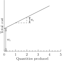
Fig. 9.1 Production cost with fixed setup cost \(w_i\).

9.1.2 Semi-continuous variables

We can also model semi-continuity of a variable \(x\in \real\),

(9.4)\[x \in 0 \cup [a,b],\]

where \(0<a\leq b\) using a double inequality

\[az \leq x \leq bz, \ z\in \{0,1\}.\]

9.1.3 Indicator constraints

Suppose we want to model the fact that a certain linear inequality must be satisfied when some other event occurs. In other words, for a binary variable \(z\) we want to model the implication

\[z=1 \implies a^Tx\leq b.\]

Suppose we know in advance an upper bound \(a^Tx-b\leq M\). Then we can write the above as a linear inequality

\[a^Tx\leq b + M(1-z).\]

Now if \(z=1\) then we forced \(a^Tx\leq b\), while for \(z=0\) the inequality is trivially satisfied and does not enforce any additional constraint on \(x\).

9.1.4 Disjunctive constraints

With a disjunctive constraint we require that at least one of the given linear constraints is satisfied, that is

\[(a_1^Tx\leq b_1) \vee (a_2^Tx\leq b_2) \vee\cdots\vee (a_k^Tx\leq b_k).\]

Introducing binary variables \(z_1,\ldots,z_k\), we can use Sec. 9.1.3 (Indicator constraints) to write a linear model

\[\begin{split}\begin{array}{l} z_1+\cdots+z_k\geq 1, \\ z_1,\ldots,z_k\in\{0,1\},\\ a_i^Tx\leq b_i+M(1-z_i),\ i=1,\ldots,k. \end{array}\end{split}\]

Note that \(z_j=1\) implies that the \(j\)-th constraint is satisfied, but not vice-versa. Achieving that effect is described in the next section.

9.1.5 Constraint satisfaction

Say we want to define an optimization model that will behave differently depending on which of the inequalities

\[a^Tx\leq b \qquad\mathrm{or}\qquad a^Tx\geq b\]

is satisfied. Suppose we have lower and upper bounds for \(a^Tx-b\) in the form of \(m\leq a^Tx-b\leq M\). Then we can write a model

(9.5)\[b+mz \leq a^Tx \leq b+M(1-z),\ z\in\{0,1\}.\]

Now observe that \(z=0\) implies \(b\leq a^Tx\leq b+M\), of which the right-hand inequality is redundant, i.e. always satisfied. Similarly, \(z=1\) implies \(b+m\leq a^Tx\leq b\). In other words \(z\) is an indicator of whether \(a^Tx\leq b\).

In practice we would relax one inequality using a small amount of slack, i.e.,

(9.6)\[b + (m-\epsilon)z + \epsilon \leq a^Tx\]

to avoid issues with classifying the equality \(a^Tx=b\).

9.1.6 Exact absolute value

In Sec. 2.2.2 (Absolute value) we showed how to model \(|x|\leq t\) as two linear inequalities. Now suppose we need to model an exact equality

(9.7)\[|x| = t.\]

It defines a non-convex set, hence it is not conic representable. If we split \(x\) into positive and negative part \(x=x^+-x^-\), where \(x^+,x^-\geq 0\), then \(|x|=x^++x^-\) as long as either \(x^+=0\) or \(x^-=0\). That last alternative can be modeled with a binary variable, and we get a model of (9.7):

(9.8)\[\begin{split}\begin{array}{rcl} x & = & x^+-x^-, \\ t & = & x^++x^-, \\ 0 & \leq & x^+,x^-, \\ x^+ & \leq & Mz, \\ x^- & \leq & M(1-z), \\ z & \in & \{0,1\}, \end{array}\end{split}\]

where the constant \(M\) is an a priori known upper bound on \(|x|\) in the problem.

9.1.7 Exact 1-norm

We can use the technique above to model the exact \(\ell_1\)-norm equality constraint

(9.9)\[\sum_{i=1}^n |x_i| = c,\]

where \(x\in\real^n\) is a decision variable and \(c\) is a constant. Such constraints arise for instance in fully invested portfolio optimizations scenarios (with short-selling). As before, we split \(x\) into a positive and negative part, using a sequence of binary variables to guarantee that at most one of them is nonzero:

(9.10)\[\begin{split}\begin{array}{rcl} x & = & x^+-x^-, \\ 0 & \leq & x^+,x^-, \\ x^+ & \leq & cz, \\ x^- & \leq & c(e-z), \\ \sum_i x^+_i +\sum_i x^-_i & = & c,\\ z & \in & \{0,1\}^n,\ x^+,x^-\in\real^n. \end{array}\end{split}\]

9.1.8 Maximum

The exact equality \(t=\max\{x_1,\ldots,x_n\}\) can be expressed by introducing a sequence of mutually exclusive indicator variables \(z_1,\ldots,z_n\), with the intention that \(z_i=1\) picks the variable \(x_i\) which actually achieves maximum. Choosing a safe bound \(M\) we get a model:

(9.11)\[\begin{split}\begin{array}{rcl} x_i&\leq & t\ \leq\ x_i+M(1-z_i),\ i=1,\ldots,n,\\ z_1+\cdots+ z_n & = & 1, \\ z & \in & \{0,1\}^n. \end{array}\end{split}\]

9.1.9 Boolean operators

Typically an indicator variable \(z\in\{0,1\}\) represents a boolean value (true/false). In this case the standard boolean operators can be implemented as linear inequalities. In the table below we assume all variables are binary.

Table 9.1 Boolean operators

Boolean	Linear
\(z= x\ \mathrm{OR}\ y\)	\(x\leq z,\ y\leq z,\ z\leq x+y\)
\(z= x\ \mathrm{AND}\ y\)	\(x\geq z,\ y\geq z,\ z+1\geq x+y\)
\(z= \mathrm{NOT}\ x\)	\(z=1-x\)
\(x\implies y\)	\(x\leq y\)
At most one of \(z_1,\ldots,z_n\) holds (SOS1, set-packing)	\(\sum_iz_i\leq 1\)
Exactly one of \(z_1,\ldots,z_n\) holds (set-partitioning)	\(\sum_iz_i= 1\)
At least one of \(z_1,\ldots,z_n\) holds (set-covering)	\(\sum_iz_i\geq 1\)
At most \(k\) of \(z_1,\ldots,z_n\) holds (cardinality)	\(\sum_iz_i\leq k\)

9.1.10 Fixed set of values

We can restrict a variable \(x\) to take on only values from a specified finite set \(\{a_1,\ldots,a_n\}\) by writing

(9.12)\[\begin{split}\begin{array}{rcl} x & = & \sum_i z_ia_i \\ z & \in & \{0,1\}^n,\\ \sum_iz_i & = & 1. \end{array}\end{split}\]

In (9.12) we essentially defined \(z_i\) to be the indicator variable of whether \(x=a_i\). In some circumstances there may be more efficient representations of a restricted set of values, for example:

• (sign) \(x\in\{-1,1\} \iff x=2z-1,\ z\in\{0,1\}\),

• (modulo) \(x\in\{1,4,7,10\} \iff x=3z+1,\ 0\leq z\leq 3,\ z\in\integral\),

• (fraction) \(x\in\{0,1/3,2/3,1\} \iff 3x=z,\ 0\leq z\leq 3, z\in\integral\),

• (gap) \(x\in(-\infty,a]\cup[b,\infty)\iff b-M(1-z)\leq x\leq a+Mz,\ z\in\{0,1\}\) for sufficiently large \(M\).

In a very similar fashion we can restrict a variable \(x\) to a finite union of intervals \(\bigcup_i [a_i,b_i]\):

(9.13)\[\begin{split}\begin{array}{l} \sum_i z_ia_i \leq x \leq \sum_i z_ib_i, \\ z \in \{0,1\}^n,\\ \sum_iz_i = 1. \end{array}\end{split}\]

9.1.11 Alternative as a bilinear equality

In the literature one often finds models containing a bilinear constraint

\[xy=0.\]

This constraint is just an algebraic formulation of the alternative \(x=0\) or \(y=0\) and therefore it can be written as a mixed-integer linear problem:

\[\begin{split}\begin{array}{rcl} |x| & \leq & Mz, \\ |y| & \leq & M(1-z), \\ z & \in & \{0,1\},\\ \end{array}\end{split}\]

for a suitable constant \(M\). The absolute value can be omitted if both \(x,y\) are nonnegative. Otherwise it can be modeled as in Sec. 2.2.2 (Absolute value).

9.1.12 Equal signs

Suppose we want to say that the variables \(x_1,\ldots,x_n\) must either be all nonnegative or all nonpositive. This can be achieved by introducing a single binary variable \(z\in\{0,1\}\) which picks one of these two alternatives:

\[-M(1-z) \leq x_i \leq Mz, \quad i=1,\ldots,n.\]

Indeed, if \(z=0\) then we have \(-M\leq x_i\leq 0\) and if \(z=1\) then \(0\leq x_i\leq M\).

9.1.13 Continuous piecewise-linear functions

Consider a continuous, univariate, piecewise-linear, non-convex function \(f:[\alpha_1,\alpha_5] \mapsto \R\) shown in Fig. 9.2. At the interval \([\alpha_j,\alpha_{j+1}]\), \(j=1,2,3,4\) we can describe the function as

\[f(x) = \lambda_j f(\alpha_j) + \lambda_{j+1} f(\alpha_{j+1})\]

where \(\lambda_j\alpha_j+\lambda_{j+1}\alpha_{j+1}=x\) and \(\lambda_j+\lambda_{j+1}=1\). If we add a constraint that only two (adjacent) variables \(\lambda_{j}, \lambda_{j+1}\) can be nonzero, we can characterize every value \(f(x)\) over the entire interval \([\alpha_1,\alpha_5]\) as some convex combination,

\[f(x) =\sum_{j=1}^4 \lambda_j f(\alpha_j).\]

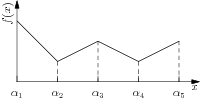
Fig. 9.2 A univariate piecewise-linear non-convex function.

The condition that only two adjacent variables can be nonzero is sometimes called an SOS2 constraint. If we introduce indicator variables \(z_i\) for each pair of adjacent variables \((\lambda_i,\lambda_{i+1})\), we can model an SOS2 constraint as:

\[\begin{split}\begin{array}{c} \lambda_1 \leq z_1, \quad \lambda_2 \leq z_1+z_2, \quad \lambda_3 \leq z_2+z_3, \quad \lambda_4 \leq z_4+z_3, \quad \lambda_5 \leq z_4\\ z_1+z_2+z_3+z_4 = 1, \quad z\in \{0,1\}^4, \end{array}\end{split}\]

so that we have \(z_j=1\implies \lambda_i=0, i\neq\{j,j+1\}\). Collectively, we can then model the epigraph \(f(x)\leq t\) as

(9.14)\[\begin{split}\begin{array}{c} x=\sum_{j=1}^n \lambda_j \alpha_j, \quad \sum_{j=1}^n \lambda_j f(\alpha_j) \leq t\\ \lambda_1 \leq z_1, \qquad \lambda_j \leq z_j + z_{j-1}, \: j=2,\dots,n-1, \qquad \lambda_n \leq z_{n-1},\\ \lambda \geq 0,\qquad \sum_{j=1}^n \lambda_j = 1, \qquad \sum_{j=1}^{n-1} z_j =1, \qquad z\in \{0,1\}^{n-1}, \end{array}\end{split}\]

for a piecewise-linear function \(f(x)\) with \(n\) terms. This approach is often called the lambda-method.

For the function in Fig. 9.2 we can reduce the number of integer variables by using a Gray encoding

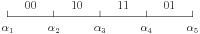
of the intervals \([\alpha_j,\alpha_{j+1}]\) and an indicator variable \(y\in \{0,1\}^2\) to represent the four different values of Gray code. We can then describe the constraints on \(\lambda\) using only two indicator variables,

\[\begin{split}\begin{array}{lll} (y_1=0) & \to & \lambda_3=0,\\ (y_1=1) & \to & \lambda_1=\lambda_5=0,\\ (y_2=0) & \to & \lambda_4=\lambda_5=0,\\ (y_2=1) & \to & \lambda_1=\lambda_2=0, \end{array}\end{split}\]

which leads to a more efficient characterization of the epigraph \(f(x)\leq t\),

\[\begin{split}\begin{array}{c} x=\sum_{j=1}^5\lambda_j \alpha_j, \quad \sum_{j=1}^5\lambda_j f(\alpha_j) \leq t,\\ \lambda_3 \leq y_1, \quad \lambda_1+\lambda_5\leq (1-y_1), \quad \lambda_4+\lambda_5\leq y_2, \quad \lambda_1+\lambda_2\leq (1-y_2),\\ \lambda\geq 0, \quad \sum_{j=1}^5\lambda_j=1, \quad y\in \{0,1\}^2, \end{array}\end{split}\]

The lambda-method can also be used to model multivariate continuous piecewise-linear non-convex functions, specified on a set of polyhedra \(P_k\). For example, for the function shown in Fig. 9.3 we can model the epigraph \(f(x)\leq t\) as

(9.15)\[\begin{split}\begin{array}{c} x=\sum_{i=1}^6 \lambda_i v_i, \qquad \sum_{i=1}^6 \lambda_i f(v_i) \leq t,\\ \lambda_1 \leq z_1 + z_2, \qquad \lambda_2\leq z_1, \qquad \lambda_3 \leq z_2+z_3,\\ \lambda_4 \leq z_1 + z_2 + z_3 + z_4, \qquad \lambda_5 \leq z_3+z_4, \qquad \lambda_6 \leq z_4,\\ \lambda \geq 0, \qquad \sum_{i=1}^6 \lambda_i = 1, \qquad \sum_{i=1}^4 z_i=1,\\ \qquad z \in \{0,1\}^4. \end{array}\end{split}\]

Note, for example, that \(z_2=1\) implies that \(\lambda_2=\lambda_5=\lambda_6=0\) and \(x=\lambda_1 v_1 + \lambda_3 v_3 + \lambda_4 v_4\).

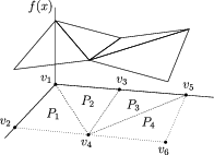
Fig. 9.3 A multivariate continuous piecewise-linear non-convex function.

9.1.14 Lower semicontinuous piecewise-linear functions

The ideas in Sec. 9.1.13 (Continuous piecewise-linear functions) can be applied to lower semicontinuous piecewise-linear functions as well. For example, consider the function shown in Fig. 9.4. If we denote the one-sided limits by \(f_{-}(c):=\lim_{x\uparrow c}f(x)\) and \(f_{+}(c):=\lim_{x\downarrow c}f(x)\), respectively, the one-sided limits, then we can describe the epigraph \(f(x)\leq t\) for the function in Fig. 9.4 as

(9.16)\[\begin{split}\begin{array}{c} x=\lambda_1 \alpha_1 + (\lambda_2+\lambda_3+\lambda_4)\alpha_2 + \lambda_5 \alpha_3,\\ \lambda_1 f(\alpha_1) + \lambda_2 f_-(\alpha_2) + \lambda_3 f(\alpha_2) + \lambda_4 f_+(\alpha_2) + \lambda_5 f(\alpha_3) \leq t, \\ \lambda_1 + \lambda_2 \leq z_1, \quad \lambda_3\leq z_2, \quad \lambda_4+\lambda_5 \leq z_3,\\ \lambda \geq 0, \qquad \sum_{i=1}^5 \lambda_i = 1, \qquad \sum_{i=1}^3 z_i=1, \qquad z \in \{0,1\}^3, \end{array}\end{split}\]

where we have a different decision variable for the intervals \([\alpha_1,\alpha_2)\), \([\alpha_2,\alpha_2]\), and \((\alpha_2,\alpha_3]\). As a special case this gives us an alternative characterization of fixed charge models considered in Sec. 9.1.1 (Implication of positivity).

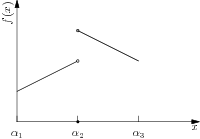
Fig. 9.4 A univariate lower semicontinuous piecewise-linear function.

9.2 Mixed integer conic case studies

9.2.1 Wireless network design

The following problem arises in wireless network design and some other applications. We want to serve \(n\) clients with \(k\) transmitters. A transmitter with range \(r_j\) can serve all clients within Euclidean distance \(r_j\) from its position. The power consumption of a transmitter with range \(r\) is proportional to \(r^\alpha\) for some fixed \(1 \leq \alpha<\infty\). The goal is to assign locations and ranges to transmitters minimizing the total power consumption while providing coverage of all \(n\) clients.

Denoting by \(x_1,\ldots,x_n\in\real^2\) locations of the clients, we can model this problem using binary decision variables \(z_{ij}\) indicating if the \(i\)-th client is covered by the \(j\)-th transmitter. This leads to a mixed-integer conic problem:

(9.17)\[\begin{split}\begin{array}{lll} \minimize & \sum_j r_j^\alpha & \\ \st & r_j \geq \|p_j-x_i\|_2 - M(1-z_{ij}), & i=1,\ldots,n,\ j=1,\ldots,k, \\ & \sum_{j} z_{ij} \geq 1, & i=1,\ldots,n, \\ & p_j\in\real^2,\ z_{ij}\in\{0,1\}. & \end{array}\end{split}\]

The objective can be realized by summing power bounds \(t_j\geq r_j^\alpha\) or by directly bounding the \(\alpha\)-norm of \((r_1,\ldots,r_k)\). The latter approach would be recommended for large \(\alpha\).

This is a type of clustering problem. For \(\alpha=1,2\), respectively, we are minimizing the perimeter and area of the covered region. In practical applications the power exponent \(\alpha\) can be as large as \(6\) depending on various factors (for instance terrain). In the linear cost model (\(\alpha=1\)) typical solutions contain a small number of huge disks covering most of the clients. For increasing \(\alpha\) large ranges are penalized more heavily and the disks tend to be more balanced.

9.2.2 Avoiding small trades

The standard portfolio optimization model admits a number of mixed-integer extensions aimed at avoiding solutions with very small trades. To fix attention consider the model

(9.18)\[\begin{split}\begin{array}{ll} \mbox{maximize} & \mu^T x\\ \mbox{subject to} & (\gamma, G^Tx)\in \Q^{n+1},\\ & e^Tx=w+e^Tx^0,\\ & x\geq 0, \end{array}\end{split}\]

with initial holdings \(x^0\), initial cash amount \(w\), expected returns \(\mu\), risk bound \(\gamma\) and decision variable \(x\). Here \(e\) is the all-ones vector. Let \(\Delta x_j=x_j-x_j^0\) denote the change of position in asset \(j\).

Transaction costs

A transaction cost involved with nonzero \(\Delta x_j\) could be modeled as

\[\begin{split}T_j(x_j) = \begin{cases} 0, & \Delta x_j = 0,\\ \alpha_j \Delta x_j + \beta_j , & \Delta x_j \neq 0, \end{cases}\end{split}\]

similarly to the problem from Example 9.1. Including transaction costs will now lead to the model:

(9.19)\[\begin{split}\begin{array}{ll} \mbox{maximize} & \mu^T x \\ \mbox{subject to} & (\gamma, G^Tx)\in \Q^{n+1},\\ & e^Tx + \alpha^T x + \beta^T z=w+e^Tx^0,\\ & x-x^0 \leq Mz,\ x^0-x\leq Mz,\\ & x\geq 0,\ z\in\{0,1\}^n, \end{array}\end{split}\]

where the binary variable \(z_j\) is an indicator of \(\Delta x_j\neq 0\). Here \(M\) is a sufficiently large constant, for instance \(M=w+e^Tx^0\) will do.

Cardinality constraints

Another option is to fix an upper bound \(k\) on the number of nonzero trades. The meaning of \(z\) is the same as before:

(9.20)\[\begin{split}\begin{array}{ll} \mbox{maximize} & \mu^T x \\ \mbox{subject to} & (\gamma, G^Tx)\in \Q^{n+1},\\ & e^Tx = w+e^Tx^0,\\ & x-x^0 \leq Mz,\ x^0-x\leq Mz,\\ & e^Tz \leq k,\\ & x\geq 0,\ z\in\{0,1\}^n. \end{array}\end{split}\]

Trading size constraints

We can also demand a lower bound on nonzero trades, that is \(|\Delta x_j|\in\{0\}\cup[a,b]\) for all \(j\). To this end we combine the techniques from Sec. 9.1.6 (Exact absolute value) and Sec. 9.1.2 (Semi-continuous variables) writing \(p_j,q_j\) for the indicators of \(\Delta x_j>0\) and \(\Delta x_j<0\), respectively:

(9.21)\[\begin{split}\begin{array}{ll} \mbox{maximize} & \mu^T x \\ \mbox{subject to} & (\gamma, G^Tx)\in \Q^{n+1},\\ & e^Tx = w+e^Tx^0,\\ & x-x^0 = x^+-x^-,\\ & x^+ \leq Mp,\ x^-\leq Mq,\\ & a(p+q)\leq x^++x^-\leq b(p+q),\\ & p+q\leq e,\\ & x,x^+,x^-\geq 0,\ p,q\in\{0,1\}^n. \end{array}\end{split}\]

9.2.3 Convex piecewise linear regression

Consider the problem of approximating the data \((x_i,y_i),\ i=1,\ldots,n\) by a piecewise linear convex function of the form

\[f(x)=\max\{a_jx+b_j,\ j=1,\ldots k\},\]

where \(k\) is the number of segments we want to consider. The quality of the fit is measured with least squares as

\[\sum_i (f(x_i)-y_i)^2.\]

Note that we do not specify the locations of nodes (breakpoints), i.e. points where \(f(x)\) changes slope. Finding them is part of the fitting problem.

As in Sec. 9.1.8 (Maximum) we introduce binary variables \(z_{ij}\) indicating that \(f(x_i)=a_jx_i+b_j\), i.e. it is the \(j\)-th linear function that achieves maximum at the point \(x_i\). Following Sec. 9.1.8 (Maximum) we now have a mixed integer conic quadratic problem

(9.22)\[\begin{split}\begin{array}{lrcll} \minimize & \|y-f\|_2 & & \\ \st & a_jx_i+b_j & \leq & f_i, & i=1,\ldots,n,\ j=1,\ldots,k,\\ & f_i & \leq & a_jx_i+b_j+M(1-z_{ij}), & i=1,\ldots,n,\ j=1,\ldots,k,\\ & \sum_j z_{ij}&= & 1, & i=1\ldots,n,\\ & z_{ij} & \in & \{0,1\},& i=1,\ldots,n,\ j=1,\ldots,k, \end{array}\end{split}\]

with variables \(a,b,f,z\), where \(M\) is a sufficiently large constant.

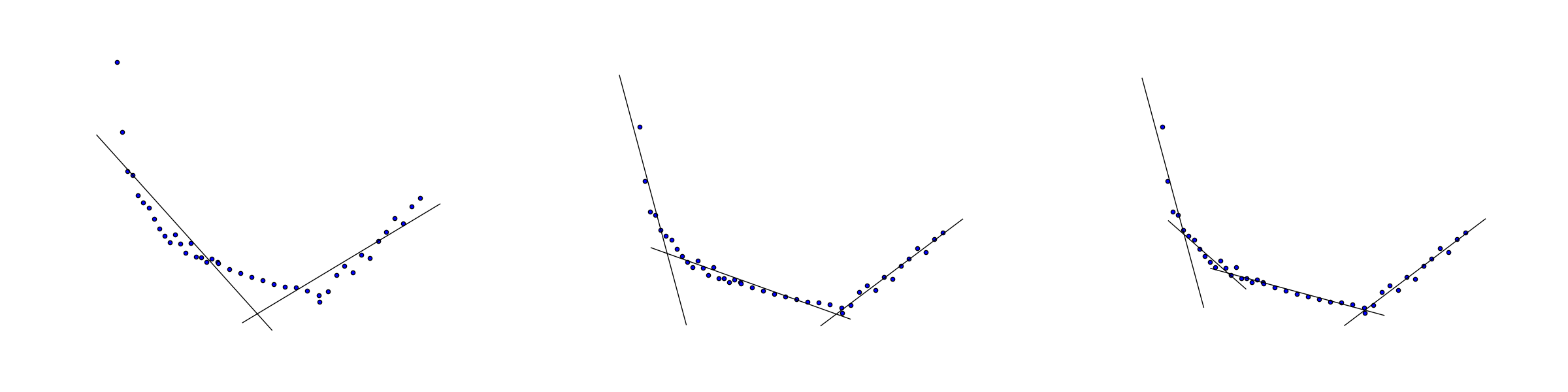
Fig. 9.5 Convex piecewise linear fit with \(k=2,3,4\) segments.

Frequently an integer model will have properties which formally follow from the problem’s constraints, but may be very hard or impossible for a mixed-integer solver to automatically deduce. It may dramatically improve efficiency to explicitly add some of them to the model. For example, we can enhance (9.22) with all inequalities of the form

\[z_{i,j+1} + z_{i+i', j} \leq 1,\]

which indicate that each linear segment covers a contiguous subset of the sample and additionally force these segments to come in the order of increasing \(j\) as \(i\) increases from left to right. The last statement is an example of symmetry breaking.