4 The power cones

So far we studied quadratic cones and their applications in modeling problems involving, directly or indirectly, quadratic terms. In this part we expand the quadratic and rotated quadratic cone family with power cones, which provide a convenient language to express models involving powers other than $2$. We must stress that although the power cones include the quadratic cones as special cases, at the current state-of-the-art they require more advanced and less efficient algorithms.

4.1 The power cone(s)

$n$-dimensional power cones form a family of convex cones parametrized by a real number $0<\alpha <1$:

(4.1)$$\begin{array}{rcl}{\mathcal{P}}_n^{\alpha ,1-\alpha }& =& \{x\in {\mathbb{R}}^n:x_1^{\alpha }{x}_2^{1-\alpha }\ge \sqrt{x_3^2+\cdots +x_n^2},x_1,x_2\ge 0\}.\end{array}$$

The constraint in the definition of ${\mathcal{P}}_n^{\alpha ,1-\alpha }$ can be expressed as a composition of two constraints, one of which is a quadratic cone:

(4.2)$$\begin{array}{r}\begin{array}{rcl}{x}_1^{\alpha }{x}_2^{1-\alpha }& \ge & |z|,\\ z& \ge & \sqrt{x_3^2+\cdots +x_n^2},\end{array}\end{array}$$

which means that the basic building block we need to consider is the three-dimensional power cone

(4.3)$$\begin{array}{rcl}{\mathcal{P}}_3^{\alpha ,1-\alpha }& =& \{x\in {\mathbb{R}}^3:x_1^{\alpha }{x}_2^{1-\alpha }\ge |x_3|,x_1,x_2\ge 0\}.\end{array}$$

More generally, we can also consider power cones with “long left-hand side”. That is, for $m<n$ and a sequence of exponents ${\alpha }_1,\dots ,{\alpha }_m$ with ${\alpha }_1+\cdots +{\alpha }_m=1$, we have the most general power cone object defined as

(4.4)$$\begin{array}{rcl}{\mathcal{P}}_n^{{\alpha }_1,\cdots ,{\alpha }_m}& =& \{x\in {\mathbb{R}}^n:\prod _{i=1}^m{x}_i^{{\alpha }_i}\ge \sqrt{\sum _{i=m+1}^n{x}_i^2},x_1,\dots ,x_m\ge 0\}.\end{array}$$

The left-hand side is nothing but the weighted geometric mean of the $x_i$, $i=1,\dots ,m$ with weights ${\alpha }_i$. In particular when all ${\alpha }_i$ are equal and there is only one element on the right-hand side we obtain as a special case the geometric mean cone:

(4.5)$${\mathcal{GM}}^n=\{x\in {\mathbb{R}}^n:{\left(\prod _{i=1}^{n-1}{x}_i\right)}^{1/(n-1)}\ge |x_n|,x_1,\dots ,x_{n-1}\ge 0\}.$$

As we will see later, both the most general power cone and the geometric mean cone can be modeled as a composition of three-dimensional cones ${\mathcal{P}}_3^{\alpha ,1-\alpha }$, so in a sense that is the basic object of interest.

There are some notable special cases we are familiar with. If we let $\alpha \to 0$ then in the limit we get ${\mathcal{P}}_n^{0,1}={\mathbb{R}}_{+}\times {\mathcal{Q}}^{n-1}$. If $\alpha =\frac{1}{2}$ then we have a rescaled version of the rotated quadratic cone, precisely:

$$(x_1,x_2,\dots ,x_n)\in {\mathcal{P}}_n^{\frac{1}{2},\frac{1}{2}}⟺(x_1/\sqrt{2},x_2/\sqrt{2},x_3,\dots ,x_n)\in {\mathcal{Q}}_{\mathit{r}}^n.$$

A gallery of three-dimensional power cones for varying $\alpha$ is shown in Fig. 4.1.

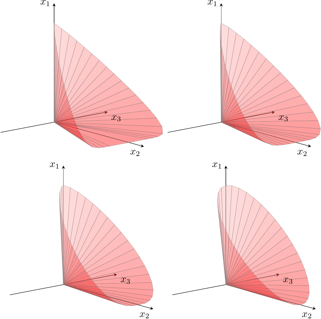
Fig. 4.1 The boundary of ${\mathcal{P}}_3^{\alpha ,1-\alpha }$ for $\alpha =0.1,0.2,0.35,0.5$.

4.2 Sets representable using the power cone

In this section we give basic examples of constraints which can be expressed using power cones.

4.2.1 Powers

For all values of $p\ne 0,1$ we can bound $x^p$ depending on the convexity of $f(x)=x^p$.

• For $p>1$ the inequality $t\ge |x{|}^p$ is equivalent to $t^{1/p}\ge |x|$ and hence corresponds to

  $$t\ge |x{|}^p⟺(t,1,x)\in {\mathcal{P}}_3^{1/p,1-1/p}.$$

  For instance $t\ge |x{|}^{1.5}$ is equivalent to $(t,1,x)\in {\mathcal{P}}_3^{2/3,1/3}$.

• For $0<p<1$ the function $f(x)=x^p$ is concave for $x\ge 0$ and so we get

  $$|t|\le x^p,x\ge 0⟺(x,1,t)\in {\mathcal{P}}_3^{p,1-p}.$$

• For $p<0$ the function $f(x)=x^p$ is convex for $x>0$ and in this range the inequality $t\ge x^p$ is equivalent to

  $$t\ge x^p⟺t^{1/(1-p)}{x}^{-p/(1-p)}\ge 1⟺(t,x,1)\in {\mathcal{P}}_3^{1/(1-p),-p/(1-p)}.$$

  For example $t\ge \frac{1}{\sqrt{x}}$ is the same as $(t,x,1)\in {\mathcal{P}}_3^{2/3,1/3}$.

4.2.2 $p$-norm cones

Let $p\ge 1$. The $p$-norm of a vector $x\in {\mathbb{R}}^n$ is $\Vert x{\Vert }_p={(|x_1{|}^p+\cdots +|x_n{|}^p)}^{1/p}$ and the $p$-norm ball of radius $t$ is defined by the inequality $\Vert x{\Vert }_p\le t$. We take the $p$-norm cone (in dimension $n+1$) to be the convex set

(4.6)$$\{(t,x)\in {\mathbb{R}}^{n+1}:t\ge \Vert x{\Vert }_p\}.$$

For $p=2$ this is precisely the quadratic cone. We can model the $p$-norm cone by writing the inequality $t\ge \Vert x{\Vert }_p$ as:

$$t\ge \sum _i|x_i{|}^p/t^{p-1}$$

and bounding each summand with a power cone. This leads to the following model:

(4.7)$$\begin{array}{r}\begin{array}{rclr}{r}_i{t}^{p-1}& \ge & |x_i{|}^p& ((r_i,t,x_i)\in {\mathcal{P}}_3^{1/p,1-1/p}),\\ \sum r_i& =& t.& \end{array}\end{array}$$

When $0<p<1$ or $p<0$ the formula for $\Vert x{\Vert }_p$ gives a concave, rather than convex function on ${\mathbb{R}}_{+}^n$ and in this case it is possible to model the set

$$\{(t,x):0\le t\le {(\sum x_i^p)}^{1/p},x_i\ge 0\},p<1,p\ne 0.$$

We leave it as an exercise (see previous subsection). The case $p=-1$ appears in Sec. 3.2.7 (Harmonic mean).

4.2.3 The most general power cone

Not all conic optimization software provides direct access to the most general version of the power cone ${\mathcal{P}}_n^{{\alpha }_1,\cdots ,{\alpha }_m}$. In this case it is good to know how to model it using the basic three-dimensional power cones ${\mathcal{P}}_3^{\alpha ,1-\alpha }$. Clearly it suffices to consider a short right-hand side, that is to model the cone

(4.8)$${\mathcal{P}}_{m+1}^{{\alpha }_1,\dots ,{\alpha }_m}=\{x_1^{{\alpha }_1}{x}_2^{{\alpha }_2}\cdots x_m^{{\alpha }_m}\ge |z|,x_1,\dots ,x_m\ge 0\},$$

where $\sum _i{\alpha }_i=1$. Denote $s={\alpha }_1+\cdots +{\alpha }_{m-1}$. We split (4.8) into two constraints

(4.9)$$\begin{array}{r}\begin{array}{rclr}{x}_1^{{\alpha }_1/s}\cdots x_{m-1}^{{\alpha }_{m-1}/s}& \ge & |t|,& x_1,\dots ,x_{m-1}\ge 0,\\ t^s{x}_m^{{\alpha }_m}& \ge & |z|,& x_m\ge 0,\end{array}\end{array}$$

and this way we expressed ${\mathcal{P}}_{m+1}^{{\alpha }_1,\dots ,{\alpha }_m}$ using two power cones ${\mathcal{P}}_m^{{\alpha }_1/s,\dots ,{\alpha }_{m-1}/s}$ and ${\mathcal{P}}_3^{s,{\alpha }_m}$. Proceeding by induction gives the desired splitting.

4.2.4 Geometric mean

The geometric mean cone ${\mathcal{GM}}^{n+1}={\mathcal{P}}_{n+1}^{1/n,\dots ,1/n}$ is a direct way to model the inequality

(4.10)$$|z|\le (x_1{x}_2\cdots x_n{)}^{1/n},$$

which corresponds to maximizing the geometric mean of the variables $x_i\ge 0$. In case this cone is not directly available to the user, tracing through the splitting (4.9) produces an equivalent representation of (4.10) using three-dimensional power cones as follows:

$$\begin{array}{r}\begin{array}{rcl}{x}_1^{1/2}{x}_2^{1/2}& \ge & |t_3|,\\ t_3^{1-1/3}{x}_3^{1/3}& \ge & |t_4|,\\ & \cdots & \\ t_{n-1}^{1-1/(n-1)}{x}_{n-1}^{1/(n-1)}& \ge & |t_n|,\\ t_n^{1-1/n}{x}_n^{1/n}& \ge & |z|.\end{array}\end{array}$$

4.2.5 Non-homogenous constraints

Every constraint of the form

$$x_1^{{\alpha }_1}{x}_2^{{\alpha }_2}\cdots x_m^{{\alpha }_m}\ge |z{|}^{\beta },x_i\ge 0,$$

where $\sum _i{\alpha }_i<\beta$ and ${\alpha }_i>0$ is equivalent to

$$(x_1,x_2,\dots ,x_m,1,z)\in {\mathcal{P}}_{m+2}^{{\alpha }_1/\beta ,\dots ,{\alpha }_m/\beta ,s}$$

with $s=1-\sum _i{\alpha }_i/\beta$.

4.3 Power cone case studies

4.3.1 Portfolio optimization with market impact

Let us go back to the Markowitz portfolio optimization problem introduced in Sec. 3.3.3 (Markowitz portfolio optimization), where we now ask to maximize expected profit subject to bounded risk in a long-only portfolio:

(4.11)$$\begin{array}{r}\begin{array}{lrcl}\text{maximize}& {\mu }^{T}x& & \\ \text{subject to}& \sqrt{x^T\mathrm{\Sigma }x}& \le & \gamma ,\\ & x_i& \ge & 0,i=1,\dots ,n,\end{array}\end{array}$$

In a realistic model we would have to consider transaction costs which decrease the expected return. In particular if a really large volume is traded then the trade itself will affect the price of the asset, a phenomenon called market impact. It is typically modeled by decreasing the expected return of $i$-th asset by a slippage cost proportional to $x^{\beta }$ for some $\beta >1$, so that the objective function changes to

$$\text{maximize}({\mu }^{T}x-\sum _i{\delta }_i{x}_i^{\beta }).$$

A popular choice is $\beta =3/2$. This objective can easily be modeled with a power cone as in Sec. 4.2 (Sets representable using the power cone):

$$\begin{array}{r}\begin{array}{lrclr}\text{maximize}& {\mu }^{T}x-{\delta }^{T}t& & & \\ \text{subject to}& (t_i,1,x_i)& \in & {\mathcal{P}}_3^{1/\beta ,1-1/\beta }& (t_i\ge x_i^{\beta }),\\ & \cdots & & & \end{array}\end{array}$$

In particular if $\beta =3/2$ the inequality $t_i\ge x_i^{3/2}$ has conic representation $(t_i,1,x_i)\in {\mathcal{P}}_3^{2/3,1/3}$.

4.3.2 Maximum volume cuboid

Suppose we have a convex, conic representable set $K\subseteq {\mathbb{R}}^n$ (for instance a polyhedron, a ball, intersections of those and so on). We would like to find a maximum volume axis-parallel cuboid inscribed in $K$. If we denote by $p\in {\mathbb{R}}^n$ the leftmost corner and by $x_1,\dots ,x_n$ the edge lengths, then this problem is equivalent to

(4.12)$$\begin{array}{r}\begin{array}{lll}\text{maximize}& t& \\ \text{subject to}& t\le (x_1\cdots x_n{)}^{1/n},& \\ & x_i\ge 0,& \\ & (p_1+e_1{x}_1,\dots ,p_n+e_n{x}_n)\in K,& \mathrm{\forall }{e}_1,\dots ,e_n\in \{0,1\},\end{array}\end{array}$$

where the last constraint states that all vertices of the cuboid are in $K$. The optimal volume is then $v=t^n$. The geometric mean cone ${\mathcal{GM}}^{n+1}$ can be used for the volume maximization constraint.

Maximizing the volume of an arbitrary (not necessarily axis-parallel) cuboid inscribed in $K$ is no longer a convex problem. However, it can be solved by maximizing the solution to (4.12) over all sets $T(K)$ where $T$ is a rotation (orthogonal matrix) in ${\mathbb{R}}^n$. In practice one can approximate the global solution by sampling sufficiently many rotations $T$ or using more advanced methods of optimization over the orthogonal group.

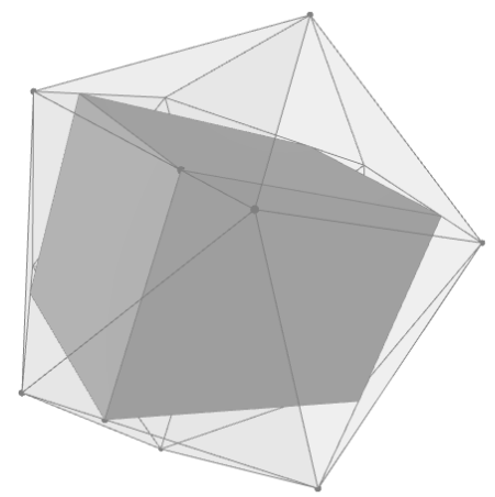
Fig. 4.2 The maximal volume cuboid inscribed in the regular icosahedron takes up approximately $0.388$ of the volume of the icosahedron (the exact value is $3(1+\sqrt{5})/25$).

4.3.3 $p$-norm geometric median

The geometric median of a sequence of points $x_1,\dots ,x_k\in {\mathbb{R}}^n$ is defined as

$${\mathrm{argmin}}_{y\in {\mathbb{R}}^n}\sum _{i=1}^k\Vert y-x_i\Vert ,$$

that is a point which minimizes the sum of distances to all the given points. Here $\Vert \cdot \Vert$ can be any norm on ${\mathbb{R}}^n$. The most classical case is the Euclidean norm, where the geometric median is the solution to the basic facility location problem minimizing total transportation cost from one depot to given destinations.

For a general $p$-norm $\Vert x{\Vert }_p$ with $1\le p<\mathrm{\infty }$ (see Sec. 4.2.2 (p-norm cones)) the geometric median is the solution to the obvious conic problem:

(4.13)$$\begin{array}{r}\begin{array}{ll}\text{minimize}& \sum _i{t}_i\\ \text{subject to}& t_i\ge \Vert y-x_i{\Vert }_p,\\ & y\in {\mathbb{R}}^n.\end{array}\end{array}$$

In Sec. 4.2.2 (p-norm cones) we showed how to model the $p$-norm bound using $n$ power cones.

The Fermat-Torricelli point of a triangle is the Euclidean geometric mean of its vertices, and a classical theorem in planar geometry (due to Torricelli, posed by Fermat), states that it is the unique point inside the triangle from which each edge is visible at the angle of ${120}^{\circ }$ (or a vertex if the triangle has an angle of ${120}^{\circ }$ or more). Using (4.13) we can compute the $p$-norm analogues of the Fermat-Torricelli point. Some examples are shown in Fig. 4.3.

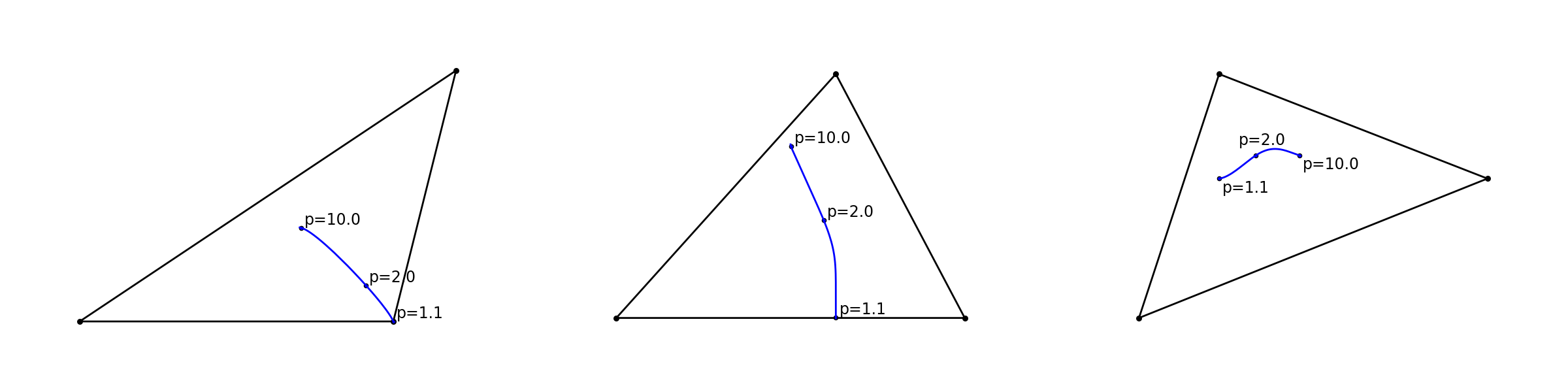
Fig. 4.3 The geometric median of three triangle vertices in various $p$-norms.

4.3.4 Maximum likelihood estimator of a convex density function

In [TV98] the problem of estimating a density function that is know in advance to be convex is considered. Here we will show that this problem can be posed as a conic optimization problem. Formally the problem is to estimate an unknown convex density function $g:{\mathbb{R}}_{+}\to {\mathbb{R}}_{+}$ given an ordered sample $y_1<y_2<\dots <y_n$ of $n$ outcomes of a distribution with density $g$.

The estimator $\tilde{g}\ge 0$ is a piecewise linear function

$$\tilde{g}:[y_1,y_n]\to {\mathbb{R}}_{+}$$

with break points at $(y_i,x_i)$, $i=1,\dots ,n$, where the variables $x_i>0$ are estimators for $g(y_i)$. The slope of the $i$-th linear segment of $\tilde{g}$ is

$$\frac{x_{i+1}-x_i}{y_{i+1}-y_i}.$$

Hence the convexity requirement leads to the constraints

$$\frac{x_{i+1}-x_i}{y_{i+1}-y_i}\le \frac{x_{i+2}-x_{i+1}}{y_{i+2}-y_{i+1}},i=1,\dots ,n-2.$$

Recall the area under the density function must be 1. Hence,

$$\sum _{i=1}^{n-1}(y_{i+1}-y_i)\left(\frac{x_{i+1}+x_i}{2}\right)=1$$

must hold. Therefore, the problem to be solved is

$$\begin{array}{r}\begin{array}{lrc}\text{maximize}& \prod _{i=1}^n{x}_i& \\ \text{subject to}& \frac{x_{i+1}-x_i}{y_{i+1}-y_i}-\frac{x_{i+2}-x_{i+1}}{y_{i+2}-y_{i+1}}& \le & 0,& i=1,\dots ,n-2,\\ & \sum _{i=1}^{n-1}(y_{i+1}-y_i)\left(\frac{x_{i+1}+x_i}{2}\right)& =& 1,\\ & x& \ge & 0.\end{array}\end{array}$$

Maximizing $\prod _{i=1}^n{x}_i$ or the geometric mean $(\prod _{i=1}^n{x}_i{)}^{\frac{1}{n}}$ will produce the same optimal solutions. Using that observation we can model the objective with the geometric mean cone ${\mathcal{GM}}^{n+1}$. Alternatively, one can use as objective $\sum _i\log x_i$ and model it using the exponential cone as in Sec. 5.2 (Modeling with the exponential cone).