12 Notation and definitions

\(\R\) and \(\integral\) denote the sets of real numbers and integers, respectively. \(\R^n\) denotes the set of \(n\)-dimensional vectors of real numbers (and similarly for \(\integral^n\) and \(\{0,1\}^n\)); in most cases we denote such vectors by lower case letters, e.g., \(a \in \R^n\). A subscripted value \(a_i\) then refers to the \(i\)-th entry in \(a\), i.e.,

\[a = (a_1, a_2, \dots, a_n).\]

The symbol \(e\) denotes the all-ones vector \(e=(1,\ldots,1)^T\), whose length always follows from the context.

All vectors are interpreted as column-vectors. For \(a,b\in \R^n\) we use the standard inner product,

\[\langle a, b \rangle := a_1 b_1 + a_2 b_2 + \dots + a_n b_n,\]

which we also write as \(a^T b := \langle a, b\rangle\). We let \(\R^{m\times n}\) denote the set of \(m\times n\) matrices, and we use upper case letters to represent them, e.g., \(B\in \R^{m\times n}\) is organized as

\[\begin{split}B = \left[\begin{array}{cccc} b_{11} & b_{12} & \dots & b_{1n}\\ b_{21} & b_{22} & \dots & b_{2n}\\ \vdots & \vdots & \ddots & \vdots\\ b_{m1} & b_{m2} & \dots & b_{mn} \end{array} \right]\end{split}\]

For matrices \(A,B\in \R^{m\times n}\) we use the inner product

\[\langle A, B \rangle := \sum_{i=1}^m \sum_{j=1}^n a_{ij} b_{ij}.\]

For a vector \(x\in \R^n\) we have

\[\begin{split}\mathbf{Diag}(x) := \left[\begin{array}{cccc} x_1 & 0 & \dots & 0\\ 0 & x_2 & \dots & 0\\ \vdots & \vdots & \ddots & \vdots \\ 0 & 0 & \dots & x_n \end{array} \right],\end{split}\]

i.e., a square matrix with \(x\) on the diagonal and zero elsewhere. Similarly, for a square matrix \(X\in\R^{n\times n}\) we have

\[\mathbf{diag}(X) := (x_{11}, x_{22}, \dots, x_{nn}).\]

A set \(S\subseteq \R^n\) is convex if and only if for any \(x, y\in S\) and \(\theta\in[0,1]\) we have

\[\theta x + (1-\theta) y \in S\]

A function \(f:\R^n \mapsto \R\) is convex if and only if its domain \(\mathbf{dom}(f)\) is convex and for all \(\theta \in [0,1]\) we have

\[f(\theta x + (1-\theta)y) \leq \theta f(x) + (1-\theta) f(y).\]

A function \(f:\R^n \mapsto \R\) is concave if and only if \(-f\) is convex. The epigraph of a function \(f:\R^n \mapsto \R\) is the set

\[\mathbf{epi}(f) := \{ (x,t) \mid x \in \mathbf{dom}(f), \: f(x) \leq t \},\]

shown in Fig. 12.1.

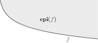
Fig. 12.1 The shaded region is the epigraph of the function \(f(x)=-\log(x)\).

Thus, minimizing over the epigraph

\[\begin{split}\begin{array}{ll} \mbox{minimize}& t\\ \mbox{subject to}& f(x) \leq t \end{array}\end{split}\]

is equivalent to minimizing \(f(x)\). Furthermore, \(f\) is convex if and only if \(\mathbf{epi}(f)\) is a convex set. Similarly, the hypograph of a function \(f:\R^n \mapsto \R\) is the set

\[\mathbf{hypo}(f) := \{ (x,t) \mid x\in \mathbf{dom}(f),\: f(x) \geq t \}.\]

Maximizing \(f\) is equivalent to maximizing over the hypograph

\[\begin{split}\begin{array}{ll} \mbox{maximize} & t\\ \mbox{subject to} & f(x) \geq t, \end{array}\end{split}\]

and \(f\) is concave if and only if \(\mathbf{hypo}(f)\) is a convex set.