10 Quadratic optimization

In this chapter we discuss convex quadratic and quadratically constrained optimization. Our discussion is fairly brief compared to the previous chapters for three reasons; (i) convex quadratic optimization is a special case of conic quadratic optimization, (ii) for most convex problems it is actually more computationally efficient to pose the problem in conic form, and (iii) duality theory (including infeasibility certificates) is much simpler for conic quadratic optimization. Therefore, we generally recommend a conic quadratic formulation, see Sec. 3 (Conic quadratic optimization) and especially Sec. 3.2.3 (Convex quadratic sets).

10.1 Quadratic objective

A standard (convex) quadratic optimization problem

(10.1)\[\begin{split}\begin{array}{ll} \mbox{minimize} & \half x^T Q x + c^T x\\ \mbox{subject to} & Ax = b,\\ & x \geq 0, \end{array}\end{split}\]

with \(Q\in\PSD^n\) is conceptually a simple extension of a standard linear optimization problem with a quadratic term \(x^T Q x\). Note the important requirement that \(Q\) is symmetric positive semidefinite; otherwise the objective function would not be convex.

10.1.1 Geometry of quadratic optimization

Quadratic optimization has a simple geometric interpretation; we minimize a convex quadratic function over a polyhedron., see Fig. 10.1. It is intuitively clear that the following different cases can occur:

• The optimal solution \(x^\star\) is at the boundary of the polyhedron (as shown in Fig. 10.1). At \(x^\star\) one of the hyperplanes is tangential to an ellipsoidal level curve.

• The optimal solution is inside the polyhedron; this occurs if the unconstrained minimizer \(\arg\min_x \half x^T Q x + c^T x=-Q^\dagger c\) (i.e., the center of the ellipsoidal level curves) is inside the polyhedron. From now on \(Q^\dagger\) denotes the pseudoinverse of \(Q\); in particular \(Q^\dagger=Q^{-1}\) if \(Q\) is positive definite.

• If the polyhedron is unbounded in the opposite direction of \(c\), and if the ellipsoid level curves are degenerate in that direction (i.e., \(Qc=0\)), then the problem is unbounded. If \(Q\in \mathcal{S}_{++}^n\), then the problem cannot be unbounded.

• The problem is infeasible, i.e., \(\{ x \mid Ax=b, \: x\geq 0 \}=\emptyset\).

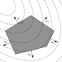
Fig. 10.1 Geometric interpretation of quadratic optimization. At the optimal point \(x^\star\) the hyperplane \(\{x\mid a_1^T x=b\}\) is tangential to an ellipsoidal level curve.

Possibly because of its simple geometric interpretation and similarity to linear optimization, quadratic optimization has been more widely adopted by optimization practitioners than conic quadratic optimization.

10.1.2 Duality in quadratic optimization

The Lagrangian function (Sec. 8.3 (Lagrangian and the dual problem)) for (10.1) is

(10.2)\[ L(x, y, s) = \half x^T Q x + x^T(c - A^Ty - s) + b^T y\]

with Lagrange multipliers \(s\in \R^n_+\), and from \(\nabla_x L(x,y,s)=0\) we get the necessary first-order optimality condition

\[Qx = A^Ty + s - c,\]

i.e. \((A^Ty+s-c)\in \mathcal{R}(Q)\). Then

\[\arg \min_x L(x,y,s) = Q^\dagger(A^Ty+s-c),\]

which can be substituted into (10.2) to give a dual function

\[\begin{split}g(y,s) = \left\{ \begin{array}{ll} b^T y - \half(A^T y + s - c) Q^\dagger (A^T y + s -c), & (A^T y + s - c) \in \mathcal{R}(Q),\\ -\infty & \text{otherwise}. \end{array} \right.\end{split}\]

Thus we get a dual problem

(10.3)\[\begin{split}\begin{array}{ll} \mbox{maximize} & b^T y - \half(A^T y + s - c) Q^\dagger (A^T y + s - c)\\ \mbox{subject to} & (A^T y + s - c) \in \mathcal{R}(Q),\\ & s \geq 0, \end{array}\end{split}\]

or alternatively, using the optimality condition \(Qx = A^T y + s - c\) we can write

(10.4)\[\begin{split}\begin{array}{ll} \mbox{maximize} & b^T y - \half x^T Q x\\ \mbox{subject to} & Qx = A^T y - c + s,\\ & s \geq 0. \end{array}\end{split}\]

Note that this is an unusual dual problem in the sense that it involves both primal and dual variables.

Weak duality, strong duality under Slater constraint qualification and Farkas infeasibility certificates work similarly as in Sec. 8 (Duality in conic optimization). In particular, note that the constraints in both (10.1) and (10.4) are linear, so Lemma 2.4 applies and we have:

1. The primal problem (10.1) is infeasible if and only if there is \(y\) such that \(A^Ty\leq 0\) and \(b^Ty> 0\).

2. The dual problem (10.4) is infeasible if and only if there is \(x\geq0\) such that \(Ax=0\), \(Qx=0\) and \(c^Tx< 0\).

10.1.3 Conic reformulation

Suppose we have a factorization \(Q=F^TF\) where \(F\in\real^{k\times n}\), which is most interesting when \(k \ll n\). Then \(x^TQx=x^TF^TFx=\|Fx\|_2^2\) and the conic quadratic reformulation of (10.1) is

(10.5)\[\begin{split}\begin{array}{ll} \mbox{minimize} & r+c^Tx\\ \mbox{subject to} & Ax=b,\\ & x\geq 0,\\ & (1,r,Fx) \in \Qr^{k+2}, \end{array}\end{split}\]

with dual problem

(10.6)\[\begin{split}\begin{array}{ll} \mbox{maximize} & b^Ty-u\\ \mbox{subject to} & -F^Tv=A^Ty-c+s,\\ & s\geq 0,\\ & (u,1,v) \in \Qr^{k+2}. \end{array}\end{split}\]

Note that in an optimal primal-dual solution we have \(r=\frac12\|Fx\|_2^2\), hence the complementary slackness for \(\Qr^{k+2}\) demands \(v=-Fx\) and \(-F^TFv=Qx\), as well as \(u=\frac12 \|v\|_2^2=\frac12 x^TQx\). This justifies why some of the dual variables in (10.6) and (10.4) have the same names - they are in fact equal, and so both the primal and dual solution to the original quadratic problem can be recovered from the primal-dual solution to the conic reformulation.

10.2 Quadratically constrained optimization

A general convex quadratically constrained quadratic optimization problem is

(10.7)\[\begin{split}\begin{array}{ll} \mbox{minimize} & \half x^T Q_0 x + c_0^T x + r_0\\ \mbox{subject to} & \half x^T Q_i x + c_i^T x + r_i \leq 0, \quad i=1,\dots,m, \end{array}\end{split}\]

where \(Q_i\in \mathcal{S}_+^n\). This corresponds to minimizing a convex quadratic function over an intersection of convex quadratic sets such as ellipsoids or affine halfspaces. Note the important requirement \(Q_i\succeq 0\) for all \(i=0,\ldots,m\), so that the objective function is convex and the constraints characterize convex sets. For example, neither of the constraints

\[\half x^T Q_i x + c_i^T x + r_i = 0,\quad \half x^T Q_i x + c_i^T x + r_i \geq 0\]

characterize convex sets, and therefore cannot be included.

10.2.1 Duality in quadratically constrained optimization

The Lagrangian function for (10.7) is

\[\begin{split}\begin{array}{ll} L(x,\lambda) & = \half x^T Q_0 x + c_0^Tx + r_0 + \sum_{i=1}^m \lambda_i \left( \half x^T Q_i x + c_i^Tx + r_i \right) \\ & = \half x^T Q(\lambda) x + c(\lambda)^T x + r(\lambda), \end{array}\end{split}\]

where

\[Q(\lambda)=Q_0 + \sum_{i=1}^m \lambda_i Q_i, \quad c(\lambda)=c_0 + \sum_{i=1}^m \lambda_i c_i, \quad r(\lambda)=r_0 + \sum_{i=1}^m \lambda_i r_i.\]

From the Lagrangian we get the first-order optimality conditions

(10.8)\[Q(\lambda) x = -c(\lambda),\]

and similar to the case of quadratic optimization we get a dual problem

(10.9)\[\begin{split}\begin{array}{ll} \mbox{maximize} & -\half c(\lambda)^T Q(\lambda)^\dagger c(\lambda) + r(\lambda)\\ \mbox{subject to} & c(\lambda) \in \mathcal{R}\left( Q(\lambda) \right),\\ & \lambda \geq 0, \end{array}\end{split}\]

or equivalently

(10.10)\[\begin{split}\begin{array}{ll} \mbox{maximize} & -\half w^T Q(\lambda) w + r(\lambda)\\ \mbox{subject to} & Q(\lambda) w = -c(\lambda),\\ & \lambda \geq 0. \end{array}\end{split}\]

Using a general version of the Schur Lemma for singular matrices, we can also write (10.9) as an equivalent semidefinite optimization problem,

(10.11)\[\begin{split}\begin{array}{ll} \mbox{maximize} & t\\ \mbox{subject to} & \left [ \begin{array}{cc}2(r(\lambda)-t) & c(\lambda)^T\\ c(\lambda) & Q(\lambda)\end{array} \right]\succeq 0,\\ & \lambda \geq 0. \end{array}\end{split}\]

Feasibility in quadratically constrained optimization is characterized by the following conditions (assuming Slater constraint qualification or other conditions to exclude ill-posed problems):

• Either the primal problem (10.7) is feasible or there exists \(\lambda \geq 0, \: \lambda \neq 0\) satisfying

  (10.12)\[\begin{split}\sum_{i=1}^m \lambda_i \left[ \begin{array}{cc} 2r_i & c_i^T \\ c_i & Q_i \end{array} \right] \succ 0.\end{split}\]

• Either the dual problem (10.10) is feasible or there exists \(x\in \R^n\) satisfying

  (10.13)\[Q_0 x = 0, \qquad c_0^T x < 0, \qquad Q_ix = 0, \qquad c_i^T x = 0, \quad i=1,\dots, m.\]

To see why the certificate proves infeasibility, suppose for instance that (10.12) and (10.7) are simultaneously satisfied. Then

\[\begin{split}0 < \sum_i\lambda_i \left[\begin{array}{c}1\\ x\end{array}\right]^T \left[\begin{array}{cc}2r_i & c_i^T\\c_i & Q_i\end{array}\right] \left[\begin{array}{c}1\\ x\end{array}\right] = 2\sum_i \lambda_i\left(\frac12 x^TQ_ix+c_i^Tx+r_i\right)\leq 0\end{split}\]

and we have a contradiction, so (10.12) certifies infeasibility.

10.2.2 Conic reformulation

If \(Q_i=F_i^TF_i\) for \(i=0,\ldots,m\), where \(F_i\in\real^{k_i\times n}\) then we get a conic quadratic reformulation of (10.7):

(10.14)\[\begin{split}\begin{array}{ll} \mbox{minimize} & t_0+c_0^Tx+r_0 \\ \mbox{subject to} & (1,t_0,F_0x)\in\Qr^{k_0+2},\\ & (1,-c_i^Tx-r_i,F_ix)\in\Qr^{k_i+2},\quad i=1,\ldots,m. \end{array}\end{split}\]

The primal and dual solution of (10.14) recovers the primal and dual solution of (10.7) similarly as for quadratic optimization in Sec. 10.1.3 (Conic reformulation). Let us see for example, how a (conic) primal infeasibility certificate for (10.14) implies an infeasibility certificate in the form (10.12). Infeasibility in (10.14) involves only the last set of conic constraints. We can derive the infeasibility certificate for those constraints from Lemma 8.3 or by directly writing the Lagrangian

\[\begin{split}\begin{array}{ll} L & = -\sum_i\left(u_i+v_i(-c_i^Tx-r_i)+w_i^TF_ix\right)\\ & = x^T\left(\sum_iv_ic_i-\sum_iF_i^Tw_i\right)+\left(\sum_iv_ir_i-\sum_iu_i\right). \end{array}\end{split}\]

The dual maximization problem is unbounded (i.e. the primal problem is infeasible) if we have

\[\begin{split}\begin{array}{ll} \sum_iv_ic_i &=\sum_iF_i^Tw_i,\\ \sum_iv_ir_i&>\sum_iu_i,\\ 2u_iv_i&\geq \|w_i\|^2,\ u_i,v_i\geq 0. \end{array}\end{split}\]

We claim that \(\lambda=v\) is an infeasibility certificate in the sense of (10.12). We can assume \(v_i>0\) for all \(i\), as otherwise \(w_i=0\) and we can take \(u_i=0\) and skip the \(i\)-th coordinate. Let \(M\) denote the matrix appearing in (10.12) with \(\lambda=v\). We show that \(M\) is positive definite:

\[\begin{split}\begin{array}{ll} [y,x]^TM[y,x] & = \sum_i\left(v_ix^TQ_ix+2v_iyc_i^Tx+2v_ir_iy^2\right)\\ & > \sum_i\left(v_i\|F_ix\|^2+2yw_i^TF_ix+2u_iy^2\right)\\ & \geq \sum_iv_i^{-1}\|v_iF_ix+yw_i\|^2 \geq 0. \end{array}\end{split}\]

10.3 Example: Factor model

Recall from Sec. 3.3.3 (Markowitz portfolio optimization) that the standard Markowitz portfolio optimization problem is

(10.15)\[\begin{split}\begin{array}{ll} \mbox{maximize} & \mu^T x\\ \mbox{subject to} & x^T \Sigma x \leq \gamma,\\ & e^T x = 1,\\ & x \geq 0, \end{array}\end{split}\]

where \(\mu\in \R^n\) is a vector of expected returns for \(n\) different assets and \(\Sigma \in \mathcal{S}_+^n\) denotes the corresponding covariance matrix. Problem (10.15) maximizes the expected return of an investment given a budget constraint and an upper bound \(\gamma\) on the allowed risk. Alternatively, we can minimize the risk given a lower bound \(\delta\) on the expected return of investment, i.e., we can solve the problem

(10.16)\[\begin{split}\begin{array}{ll} \mbox{minimize} & x^T \Sigma x\\ \mbox{subject to} & \mu^T x \geq \delta,\\ & e^T x = 1,\\ & x \geq 0. \end{array}\end{split}\]

Both problems (10.15) and (10.16) are equivalent in the sense that they describe the same Pareto-optimal trade-off curve by varying \(\delta\) and \(\gamma\).

Next consider a factorization

(10.17)\[ \Sigma = V^T V\]

for some \(V\in\R^{k\times n}\). We can then rewrite both problems (10.15) and (10.16) in conic quadratic form as

(10.18)\[\begin{split}\begin{array}{ll} \mbox{maximize} & \mu^T x\\ \mbox{subject to} & (1/2, \gamma, Vx) \in \mathcal{Q}_r^{k+2},\\ & e^Tx = 1,\\ & x \geq 0, \end{array}\end{split}\]

and

(10.19)\[\begin{split}\begin{array}{ll} \mbox{minimize} & t\\ \mbox{subject to} & (1/2, t, Vx) \in \mathcal{Q}_r^{k+2},\\ & \mu^T x \geq \delta,\\ & e^Tx = 1,\\ & x \geq 0, \end{array}\end{split}\]

respectively. Given \(\Sigma\succ 0\), we may always compute a factorization (10.17) where \(V\) is upper-triangular (Cholesky factor). In this case \(k=n\), i.e., \(V\in\R^{n\times n}\), so there is little difference in complexity between the conic and quadratic formulations. However, in practice, better choices of \(V\) are either known or readily available. We mention two examples.

Data matrix

\(\Sigma\) might be specified directly in the form (10.17), where \(V\) is a normalized data-matrix with \(k\) observations of market data (for example daily returns) of the \(n\) assets. When the observation horizon \(k\) is shorter than \(n\), which is typically the case, the conic representation is both more parsimonious and has better numerical properties.

Factor model

For a factor model we have

\[\Sigma = D + U^T R U\]

where \(D=\Diag(w)\) is a diagonal matrix, \(U \in \R^{k\times n}\) represents the exposure of assets to risk factors and \(R\in \real^{k\times k}\) is the covariance matrix of factors. Importantly, we normally have a small number of factors (\(k\ll n\)), so it is computationally much cheaper to find a Cholesky decomposition \(R=F^TF\) with \(F\in\real^{k\times k}\). This combined gives us \(\Sigma=V^TV\) for

\[\begin{split}V = \left [ \begin{array}{c}D^{1/2} \\ FU\end{array}\right ]\end{split}\]

of dimensions \((n+k)\times n\). The dimensions of \(V\) are larger than the dimensions of the Cholesky factors of \(\Sigma\), but \(V\) is very sparse, which usually results in a significant reduction of solution time. The resulting risk minimization conic problem can ultimately be written as:

(10.20)\[\begin{split}\begin{array}{ll} \mbox{minimize} & t\\ \mbox{subject to} & \left(1/2, t, \left[\begin{array}{c}D^{1/2}\\ FU\end{array}\right]x \right) \in \mathcal{Q}_r^{n+k+2},\\ & \mu^T x \geq \delta,\\ & e^Tx = 1,\\ & x \geq 0. \end{array}\end{split}\]