5 Exponential cone optimization

So far we discussed optimization problems involving the major “polynomial” families of cones: linear, quadratic and power cones. In this chapter we introduce a single new object, namely the three-dimensional exponential cone, together with examples and applications. The exponential cone can be used to model a variety of constraints involving exponentials and logarithms.

5.1 Exponential cone

The exponential cone is a convex subset of ${\mathbb{R}}^3$ defined as

(5.1)$$\begin{array}{r}\begin{array}{rcl}{K}_{\exp }& =& \{(x_1,x_2,x_3):x_1\ge x_2{e}^{x_3/x_2},x_2>0\}\cup \\ & & \{(x_1,0,x_3):x_1\ge 0,x_3\le 0\}.\end{array}\end{array}$$

Thus the exponential cone is the closure in ${\mathbb{R}}^3$ of the set of points which satisfy

(5.2)$$x_1\ge x_2{e}^{x_3/x_2},x_1,x_2>0.$$

When working with logarithms, a convenient reformulation of (5.2) is

(5.3)$$x_3\le x_2\log (x_1/x_2),x_1,x_2>0.$$

Alternatively, one can write the same condition as

$$x_1/x_2\ge e^{x_3/x_2},x_1,x_2>0,$$

which immediately shows that $K_{\exp }$ is in fact a cone, i.e. $\alpha x\in K_{\exp }$ for $x\in K_{\exp }$ and $\alpha \ge 0$. Convexity of $K_{\exp }$ follows from the fact that the Hessian of $f(x,y)=y\exp (x/y)$, namely

$$\begin{array}{r}{D}^2(f)=e^{x/y}\left[\begin{array}{cc}{y}^{-1}& -x{y}^{-2}\\ -x{y}^{-2}& x^2{y}^{-3}\end{array}\right]\end{array}$$

is positive semidefinite for $y>0$.

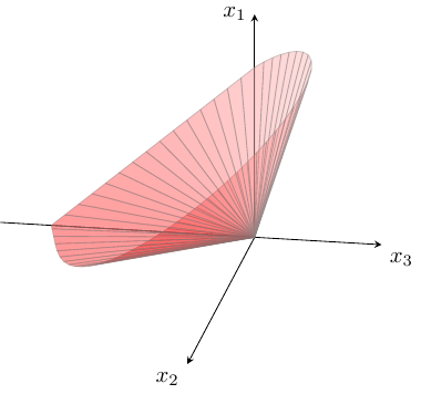
Fig. 5.1 The boundary of the exponential cone $K_{\exp }$.

5.2 Modeling with the exponential cone

Extending the conic optimization toolbox with the exponential cone leads to new types of constraint building blocks and new types of representable sets. In this section we list the basic operations available using the exponential cone.

5.2.1 Exponential

The epigraph $t\ge e^x$ is a section of $K_{\exp }$:

(5.4)$$t\ge e^x⟺(t,1,x)\in K_{\exp }.$$

5.2.2 Logarithm

Similarly, we can express the hypograph $t\le \log x,x\ge 0$:

(5.5)$$t\le \log x⟺(x,1,t)\in K_{\exp }.$$

5.2.3 Entropy

The entropy function $H(x)=-x\log x$ can be maximized using the following representation which follows directly from (5.3):

(5.6)$$t\le -x\log x⟺t\le x\log (1/x)⟺(1,x,t)\in K_{\exp }.$$

5.2.4 Relative entropy

The relative entropy or Kullback-Leiber divergence of two probability distributions is defined in terms of the function $D(x,y)=x\log (x/y)$. It is convex, and the minimization problem $t\ge D(x,y)$ is equivalent to

(5.7)$$t\ge D(x,y)⟺-t\le x\log (y/x)⟺(y,x,-t)\in K_{\exp }.$$

Because of this reparametrization the exponential cone is also referred to as the relative entropy cone, leading to a class of problems known as REPs (relative entropy problems). Having the relative entropy function available makes it possible to express epigraphs of other functions appearing in REPs, for instance:

$$x\log (1+x/y)=D(x+y,y)+D(y,x+y).$$

5.2.5 Softplus function

In neural networks the function $f(x)=\log (1+e^x)$, known as the softplus function, is used as an analytic approximation to the rectifier activation function $r(x)=x^{+}=max(0,x)$. The softplus function is convex and we can express its epigraph $t\ge \log (1+e^x)$ by combining two exponential cones. Note that

$$t\ge \log (1+e^x)⟺e^{x-t}+e^{-t}\le 1$$

and therefore $t\ge \log (1+e^x)$ is equivalent to the following set of conic constraints:

(5.8)$$\begin{array}{r}\begin{array}{rcl}u+v& \le & 1,\\ (u,1,x-t)& \in & K_{\exp },\\ (v,1,-t)& \in & K_{\exp }.\end{array}\end{array}$$

5.2.6 Log-sum-exp

We can generalize the previous example to a log-sum-exp (logarithm of sum of exponentials) expression

$$t\ge \log (e^{x_1}+\cdots +e^{x_n}).$$

This is equivalent to the inequality

$$e^{x_1-t}+\cdots +e^{x_n-t}\le 1,$$

and so it can be modeled as follows:

(5.9)$$\begin{array}{r}\begin{array}{rcl}\sum u_i& \le & 1,\\ (u_i,1,x_i-t)& \in & K_{\exp },i=1,\dots ,n.\end{array}\end{array}$$

5.2.7 Log-sum-inv

The following type of bound has applications in capacity optimization for wireless network design:

$$t\ge \log (\frac{1}{x_1}+\cdots +\frac{1}{x_n}),x_i>0.$$

Since the logarithm is increasing, we can model this using a log-sum-exp and an exponential as:

$$\begin{array}{r}\begin{array}{l}t\ge \log (e^{y_1}+\cdots +e^{y_n}),\\ x_i\ge e^{-y_i},i=1,\dots ,n.\end{array}\end{array}$$

Alternatively, one can also rewrite the original constraint in equivalent form:

$$e^{-t}\le s\le {(\frac{1}{x_1}+\cdots +\frac{1}{x_n})}^{-1},x_i>0.$$

and then model the right-hand side inequality using the technique from Sec. 3.2.7 (Harmonic mean). This approach requires only one exponential cone.

5.2.8 Arbitrary exponential

The inequality

$$t\ge a_1^{x_1}{a}_2^{x_2}\cdots a_n^{x_n},$$

where $a_i$ are arbitrary positive constants, is of course equivalent to

$$t\ge \exp (\sum _i{x}_i\log a_i)$$

and therefore to $(t,1,\sum _i{x}_i\log a_i)\in K_{\exp }$.

5.2.9 Lambert W-function

The Lambert function $W:{\mathbb{R}}_{+}\to {\mathbb{R}}_{+}$ is the unique function satisfying the identity

$$W(x)e^{W(x)}=x.$$

It is the real branch of a more general function which appears in applications such as diode modeling. The $W$ function is concave. Although there is no explicit analytic formula for $W(x)$, the hypograph $\{(x,t):0\le x,0\le t\le W(x)\}$ has an equivalent description:

$$x\ge t{e}^t=t{e}^{t^2/t}$$

and so it can be modeled with a mix of exponential and quadratic cones (see Sec. 3.1.2 (Rotated quadratic cones)):

(5.10)$$\begin{array}{r}\begin{array}{rclr}(x,t,u)& \in & K_{\exp },& (x\ge t\exp (u/t)),\\ (1/2,u,t)& \in & {\mathcal{Q}}_{\mathit{r}},& (u\ge t^2).\end{array}\end{array}$$

5.2.10 Other simple sets

Here are a few more typical sets which can be expressed using the exponential and quadratic cones. The presentations should be self-explanatory; we leave the simple verifications to the reader.

Table 5.1 Sets representable with the exponential cone

Set	Conic representation
$t\ge (\log x{)}^2,0<x\le 1$	$(\frac{1}{2},t,u)\in {\mathcal{Q}}_{\mathit{r}}^3,(x,1,u)\in K_{\exp },x\le 1$
$t\le \log \log x,x>1$	$(u,1,t)\in K_{\exp },(x,1,u)\in K_{\exp }$
$t\ge (\log x{)}^{-1},x>1$	$(u,t,\sqrt{2})\in {\mathcal{Q}}_{\mathit{r}}^3,(x,1,u)\in K_{\exp }$
$t\le \sqrt{\log x},x>1$	$(\frac{1}{2},u,t)\in {\mathcal{Q}}_{\mathit{r}}^3,(x,1,u)\in K_{\exp }$
$t\le \sqrt{x\log x},x>1$	$(x,u,\sqrt{2}t)\in {\mathcal{Q}}_{\mathit{r}}^3,(x,1,u)\in K_{\exp }$
$t\le \log (1-1/x),x>1$	$(x,u,\sqrt{2})\in {\mathcal{Q}}_{\mathit{r}}^3,(1-u,1,t)\in K_{\exp }$
$t\ge \log (1+1/x),x>0$	$(x+1,u,\sqrt{2})\in {\mathcal{Q}}_{\mathit{r}}^3,(1-u,1,-t)\in K_{\exp }$

5.3 Geometric programming

Geometric optimization problems form a family of optimization problems with objective and constraints in special polynomial form. It is a rich class of problems solved by reformulating in logarithmic-exponential form, and thus a major area of applications for the exponential cone $K_{\exp }$. Geometric programming is used in circuit design, chemical engineering, mechanical engineering and finance, just to mention a few applications. We refer to [BKVH07] for a survey and extensive bibliography.

5.3.1 Definition and basic examples

A monomial is a real valued function of the form

(5.11)$$f(x_1,\dots ,x_n)=c{x}_1^{a_1}{x}_2^{a_2}\cdots x_n^{a_n},$$

where the exponents $a_i$ are arbitrary real numbers and $c>0$. A posynomial (positive polynomial) is a sum of monomials. Thus the difference between a posynomial and a standard notion of a multi-variate polynomial known from algebra or calculus is that (i) posynomials can have arbitrary exponents, not just integers, but (ii) they can only have positive coefficients.

For example, the following functions are monomials (in variables $x,y,z$):

(5.12)$$xy,2x^{1.5}{y}^{-1}{x}^{0.3},3\sqrt{xy/z},1$$

and the following are examples of posynomials:

(5.13)$$2x+yz,1.5x^{3}z+5/y,(x^2{y}^2+3z^{-0.3}{)}^4+1.$$

A geometric program (GP) is an optimization problem of the form

(5.14)$$\begin{array}{r}\begin{array}{lll}\text{minimize}& f_0(x)& \\ \text{subject to}& f_i(x)\le 1,& i=1,\dots ,m,\\ & x_j>0,& j=1,\dots ,n,\end{array}\end{array}$$

where $f_0,\dots ,f_m$ are posynomials and $x=(x_1,\dots ,x_n)$ is the variable vector.

A geometric program (5.14) can be modeled in exponential conic form by making a substitution

$$x_j=e^{y_j},j=1,\dots ,n.$$

Under this substitution a monomial of the form (5.11) becomes

$$c{e}^{a_1{y}_1}{e}^{a_2{y}_2}\cdots e^{a_n{y}_n}=\exp (a_{\ast }^{T}y+\log c)$$

for $a_{\ast }=(a_1,\dots ,a_n)$. Consequently, the optimization problem (5.14) takes an equivalent form

(5.15)$$\begin{array}{r}\begin{array}{lrcl}\text{minimize}t& & & \\ \text{subject to}& \log (\sum _k\exp (a_{0,k,\ast }^{T}y+\log c_{0,k}))& \le & t,\\ & \log (\sum _k\exp (a_{i,k,\ast }^{T}y+\log c_{i,k}))& \le & 0,i=1,\dots ,m,\end{array}\end{array}$$

where $a_{i,k}\in {\mathbb{R}}^n$ and $c_{i,k}\in \mathbb{R}$ for all $i,k$. These are now log-sum-exp constraints we already discussed in Sec. 5.2.6 (Log-sum-exp). In particular, the problem (5.15) is convex, as opposed to the posynomial formulation (5.14).

Example

We demonstrate this reduction on a simple example. Take the geometric problem

$$\begin{array}{r}\begin{array}{lrcl}\text{minimize}& x+y^{2}z& & \\ \text{subject to}& 0.1\sqrt{x}+2y^{-1}& \le & 1,\\ & z^{-1}+y{x}^{-2}& \le & 1.\end{array}\end{array}$$

By substituting $x=e^u$, $y=e^v$, $z=e^w$ we get

$$\begin{array}{r}\begin{array}{lrcl}\text{minimize}t& & & \\ \text{subject to}& \log (e^u+e^{2v+w})& \le & t,\\ & \log (e^{0.5u+\log 0.1}+e^{-v+\log 2})& \le & 0,\\ & \log (e^{-w}+e^{v-2u})& \le & 0.\end{array}\end{array}$$

and using the log-sum-exp reduction from Sec. 5.2.6 (Log-sum-exp) we write an explicit conic problem:

$$\begin{array}{r}\begin{array}{ll}\text{minimize}t& \\ \text{subject to}& (p_1,1,u-t),(q_1,1,2v+w-t)\in K_{\exp },& p_1+q_1\le 1,\\ & (p_2,1,0.5u+\log 0.1),(q_2,1,-v+\log 2)\in K_{\exp },& p_2+q_2\le 1,\\ & (p_3,1,-w),(q_3,1,v-2u)\in K_{\exp },& p_3+q_3\le 1.\end{array}\end{array}$$

Solving this problem yields $(x,y,z)\approx (3.14,2.43,1.32)$.

5.3.2 Generalized geometric models

In this section we briefly discuss more general types of constraints which can be modeled with geometric programs.

Monomials

If $m(x)$ is a monomial then the constraint $m(x)=c$ is equivalent to two posynomial inequalities $m(x)c^{-1}\le 1$ and $m(x{)}^{-1}c\le 1$, so it can be expressed in the language of geometric programs. In practice it should be added to the model (5.15) as a linear constraint

$$\sum _k{a}_k{y}_k=\log c.$$

Monomial inequalities $m(x)\le c$ and $m(x)\ge c$ should similarly be modeled as linear inequalities in the $y_i$ variables.

In similar vein, if $f(x)$ is a posynomial and $m(x)$ is a monomial then $f(x)\le m(x)$ is still a posynomial inequality because it can be written as $f(x)m(x{)}^{-1}\le 1$.

It also means that we can add lower and upper variable bounds: $0<c_1\le x\le c_2$ is equivalent to $x^{-1}{c}_1\le 1$ and $c_2^{-1}x\le 1$.

Products and positive powers

Expressions involving products and positive powers (possibly iterated) of posynomials can again be modeled with posynomials. For example, a constraint such as

$$((x{y}^2+z{)}^{0.3}+y)(1/x+1/y{)}^{2.2}\le 1$$

can be replaced with

$$x{y}^2+z\le t,t^{0.3}+y\le u,x^{-1}+y^{-1}\le v,u{v}^{2.2}\le 1.$$

Other transformations and extensions

• If $f_1,f_2$ are already expressed by posynomials then $max\{f_1(x),f_2(x)\}\le t$ is clearly equivalent to $f_1(x)\le t$ and $f_2(x)\le t$. Hence we can add the maximum operator to the list of building blocks for geometric programs.

• If $f,g$ are posynomials, $m$ is a monomial and we know that $m(x)\ge g(x)$ then the constraint $\frac{f(x)}{m(x)-g(x)}\le t$ is equivalent to $t^{-1}f(x)m(x{)}^{-1}+g(x)m(x{)}^{-1}\le 1$.

• The objective function of a geometric program (5.14) can be extended to include other terms, for example:

  $$\text{minimize}{f}_0(x)+\sum _k\log m_k(x)$$

  where $m_k(x)$ are monomials. After the change of variables $x=e^y$ we get a slightly modified version of (5.15):

  $$\begin{array}{r}\begin{array}{lrcl}\text{minimize}& t+b^{T}y& & \\ \text{subject to}& \sum _k\exp (a_{0,k,\ast }^{T}y+\log c_{0,k})& \le & t,\\ & \log (\sum _k\exp (a_{i,k,\ast }^{T}y+\log c_{i,k}))& \le & 0,i=1,\dots ,m,\end{array}\end{array}$$

  (note the lack of one logarithm) which can still be expressed with exponential cones.

5.3.3 Geometric programming case studies

Frobenius norm diagonal scaling

Suppose we have a matrix $M\in {\mathbb{R}}^{n\times n}$ and we want to rescale the coordinate system using a diagonal matrix $D=\mathbf{Diag}(d_1,\dots ,d_n)$ with $d_i>0$. In the new basis the linear transformation given by $M$ will now be described by the matrix $DM{D}^{-1}=(d_i{M}_{ij}{d}_j^{-1}{)}_{i,j}$. To choose $D$ which leads to a “small” rescaling we can for example minimize the Frobenius norm

$$\Vert DM{D}^{-1}{\Vert }_F^2=\sum _{ij}{((DM{D}^{-1}{)}_{ij})}^2=\sum _{ij}{M}_{ij}^2{d}_i^2{d}_j^{-2}.$$

Minimizing the last sum is an example of a geometric program with variables $d_i$ (and without constraints).

Maximum likelihood estimation

Geometric programs appear naturally in connection with maximum likelihood estimation of parameters of random distributions. Consider a simple example. Suppose we have two biased coins, with head probabilities $p$ and $2p$, respectively. We toss both coins and count the total number of heads. Given that, in the long run, we observed $i$ heads $n_i$ times for $i=0,1,2$, estimate the value of $p$.

The probability of obtaining the given outcome equals

$$(\genfrac{}{}{0ex}{}{n_0+n_1+n_2}{n_0})(\genfrac{}{}{0ex}{}{n_1+n_2}{n_1})(p\cdot 2p{)}^{n_2}{(p(1-2p)+2p(1-p))}^{n_1}{((1-p)(1-2p))}^{n_0},$$

and, up to constant factors, maximizing that expression is equivalent to solving the problem

$$\begin{array}{r}\begin{array}{lrcl}\text{maximize}& p^{2n_2+n_1}{s}^{n_1}{q}^{n_0}{r}^{n_0}& & \\ \text{subject to}& q& \le & 1-p,\\ & r& \le & 1-2p,\\ & s& \le & 3-4p,\end{array}\end{array}$$

or, as a geometric problem:

$$\begin{array}{r}\begin{array}{lrcl}\text{minimize}& p^{-2n_2-n_1}{s}^{-n_1}{q}^{-n_0}{r}^{-n_0}& & \\ \text{subject to}& q+p& \le & 1,\\ & r+2p& \le & 1,\\ & \frac{1}{3}s+\frac{4}{3}p& \le & 1.\end{array}\end{array}$$

For example, if $(n_0,n_1,n_2)=(30,53,16)$ then the above problem solves with $p=0.29$.

An Olympiad problem

The 26th Vojtěch Jarník International Mathematical Competition, Ostrava 2016. Let $a,b,c$ be positive real numbers with $a+b+c=1$. Prove that

$$(\frac{1}{a}+\frac{1}{bc})(\frac{1}{b}+\frac{1}{ac})(\frac{1}{c}+\frac{1}{ab})\ge 1728$$

Using the tricks introduced in Sec. 5.3.2 (Generalized geometric models) we formulate this problem as a geometric program:

$$\begin{array}{r}\begin{array}{lrcl}\text{minimize}& pqr& & \\ \text{subject to}& p^{-1}{a}^{-1}+p^{-1}{b}^{-1}{c}^{-1}& \le & 1,\\ & q^{-1}{b}^{-1}+q^{-1}{a}^{-1}{c}^{-1}& \le & 1,\\ & r^{-1}{c}^{-1}+r^{-1}{a}^{-1}{b}^{-1}& \le & 1,\\ & a+b+c& \le & 1.\end{array}\end{array}$$

Unsurprisingly, the optimal value of this program is $1728$, achieved for $(a,b,c,p,q,r)=(\frac{1}{3},\frac{1}{3},\frac{1}{3},12,12,12)$.

Power control and rate allocation in wireless networks

We consider a basic wireless network power control problem. In a wireless network with $n$ logical transmitter-receiver pairs if the power output of transmitter $j$ is $p_j$ then the power received by receiver $i$ is $G_{ij}{p}_j$, where $G_{ij}$ models path gain and fading effects. If the $i$-th receiver’s own noise is ${\sigma }_i$ then the signal-to-interference-plus-noise (SINR) ratio of receiver $i$ is given by

(5.16)$$s_i=\frac{G_{ii}{p}_i}{{\sigma }_i+\sum _{j\ne i}{G}_{ij}{p}_j}.$$

Maximizing the minimal SINR over all receivers ($max\underset{i}{min}{s}_i$), subject to bounded power output of the transmitters, is equivalent to the geometric program with variables $p_1,\dots ,p_n,t$:

(5.17)$$\begin{array}{r}\begin{array}{lrcr}\text{minimize}& t^{-1}& & \\ \text{subject to}& p_{\min }\le p_j\le p_{\max },& & j=1,\dots ,n,\\ & t({\sigma }_i+\sum _{j\ne i}{G}_{ij}{p}_j)G_{ii}^{-1}{p}_i^{-1}& \le & 1,i=1,\dots ,n.\end{array}\end{array}$$

In the low-SNR regime the problem of system rate maximization is approximated by the problem of maximizing $\sum _i\log s_i$, or equivalently minimizing $\prod _i{s}_i^{-1}$. This is a geometric problem with variables $p_i,s_i$:

(5.18)$$\begin{array}{r}\begin{array}{lrcr}\text{minimize}& s_1^{-1}\cdot \cdots s_n^{-1}& & \\ \text{subject to}& p_{\min }\le p_j\le p_{\max },& & j=1,\dots ,n,\\ & s_i({\sigma }_i+\sum _{j\ne i}{G}_{ij}{p}_j)G_{ii}^{-1}{p}_i^{-1}& \le & 1,i=1,\dots ,n.\end{array}\end{array}$$

For more information and examples see [BKVH07].

5.4 Exponential cone case studies

In this section we introduce some practical optimization problems where the exponential cone comes in handy.

5.4.1 Risk parity portfolio

Consider a simple version of the Markowitz portfolio optimization problem introduced in Sec. 3.3.3 (Markowitz portfolio optimization), where we simply ask to minimize the risk $r(x)=\sqrt{x^T\mathrm{\Sigma }x}$ of a fully-invested long-only portfolio:

(5.19)$$\begin{array}{r}\begin{array}{lrcl}\text{minimize}& \sqrt{x^T\mathrm{\Sigma }x}& & \\ \text{subject to}& \sum _{i=1}^n{x}_i& =& 1,\\ & x_i& \ge & 0,i=1,\dots ,n,\end{array}\end{array}$$

where $\mathrm{\Sigma }$ is a symmetric positive definite covariance matrix. We can derive from the first-order optimality conditions that the solution to (5.19) satisfies $\frac{\partial r}{\partial x_i}=\frac{\partial r}{\partial x_j}$ whenever $x_i,x_j>0$, i.e. marginal risk contributions of positively invested assets are equal. In practice this often leads to concentrated portfolios, whereas it would benefit diversification to consider portfolios where all assets have the same total contribution to risk:

(5.20)$$x_i\frac{\partial r}{\partial x_i}=x_j\frac{\partial r}{\partial x_j},i,j=1,\dots ,n.$$

We call (5.20) the risk parity condition. It indeed models equal risk contribution from all the assets, because as one can easily check $\frac{\partial r}{\partial x_i}=\frac{(\mathrm{\Sigma }x{)}_i}{\sqrt{x^T\mathrm{\Sigma }x}}$ and

$$r(x)=\sum _i{x}_i\frac{\partial r}{\partial x_i}.$$

Risk parity portfolios satisfying condition (5.20) can be found with an auxiliary optimization problem:

(5.21)$$\begin{array}{r}\begin{array}{lrl}\text{minimize}& \sqrt{x^T\mathrm{\Sigma }x}-c\sum _i\log x_i& \\ \text{subject to}& x_i>0,& i=1,\dots ,n,\end{array}\end{array}$$

for any $c>0$. More precisely, the gradient of the objective function in (5.21) is zero when $\frac{\partial r}{\partial x_i}=c/x_i$ for all $i$, implying the parity condition (5.20) holds. Since (5.20) is scale-invariant, we can rescale any solution of (5.21) and get a fully-invested risk parity portfolio with $\sum _i{x}_i=1$.

The conic form of problem (5.21) is:

(5.22)$$\begin{array}{r}\begin{array}{lrclr}\text{minimize}& t-c{e}^{T}s& & & \\ \text{subject to}& (t,{\mathrm{\Sigma }}^{1/2}x)& \in & {\mathcal{Q}}^{n+1},& (t\ge \sqrt{x^T\mathrm{\Sigma }x}),\\ & (x_i,1,s_i)& \in & K_{\exp },& (s_i\le \log x_i).\end{array}\end{array}$$

5.4.2 Entropy maximization

A general entropy maximization problem has the form

(5.23)$$\begin{array}{r}\begin{array}{lrcl}\text{maximize}& -\sum _i{p}_i\log p_i& & \\ \text{subject to}& \sum _i{p}_i& =& 1,\\ & p_i& \ge & 0,\\ & p& \in & \mathcal{I},\end{array}\end{array}$$

where $\mathcal{I}$ defines additional constraints on the probability distribution $p$ (these are known as prior information). In the absence of complete information about $p$ the maximum entropy principle of Jaynes posits to choose the distribution which maximizes uncertainty, that is entropy, subject to what is known. Practitioners think of the solution to (5.23) as the most random or most conservative of distributions consistent with $\mathcal{I}$.

Maximization of the entropy function $H(x)=-x\log x$ was explained in Sec. 5.2 (Modeling with the exponential cone).

Often one has an a priori distribution $q$, and one tries to minimize the distance between $p$ and $q$, while remaining consistent with $\mathcal{I}$. In this case it is standard to minimize the Kullback-Leiber divergence

$${\mathcal{D}}_{KL}(p||q)=\sum _i{p}_i\log p_i/q_i$$

which leads to an optimization problem

(5.24)$$\begin{array}{r}\begin{array}{lrcl}\text{minimize}& \sum _i{p}_i\log p_i/q_i& & \\ \text{subject to}& \sum _i{p}_i& =& 1,\\ & p_i& \ge & 0,\\ & p& \in & \mathcal{I}.\end{array}\end{array}$$

5.4.3 Hitting time of a linear system

Consider a linear dynamical system

(5.25)$${\mathbf{x}}^{\prime }(t)=A\mathbf{x}(t)$$

where we assume for simplicity that $A=\mathbf{Diag}(a_1,\dots ,a_n)$ with $a_i<0$ with initial condition $\mathbf{x}(0{)}_i=x_i$. The resulting dynamical system $\mathbf{x}(t)=\mathbf{x}(0)\exp (At)$ converges to $0$ and one can ask, for instance, for the time it takes to approach the limit up to distance $\epsilon$. The resulting optimization problem is

$$\begin{array}{r}\begin{array}{lrcl}\text{minimize}& t& & \\ \text{subject to}& \sqrt{\sum _i{(x_i\exp (a_{i}t))}^2}& \le & \epsilon ,\end{array}\end{array}$$

with the following conic form, where the variables are $t,q_1,\dots ,q_n$:

$$\begin{array}{r}\begin{array}{lrcl}\text{minimize}& t& & \\ \text{subject to}& (\epsilon ,x_1{q}_1,\dots ,x_n{q}_n)& \in & {\mathcal{Q}}^{n+1},\\ & (q_i,1,a_{i}t)& \in & K_{\exp },i=1,\dots ,n.\end{array}\end{array}$$

See Fig. 5.2 for an example. Other criteria for the target set of the trajectories are also possible. For example, polyhedral constraints

$$c^T\mathbf{x}\le d,c\in {\mathbb{R}}_{+}^n,d\in {\mathbb{R}}_{+}$$

are also expressible in exponential conic form for starting points $\mathbf{x}(0)\in {\mathbb{R}}_{+}^n$, since they correspond to log-sum-exp constraints of the form

$$\log (\sum _i\exp (a_i{\mathbf{x}}_i+\log (c_i{x}_i)))\le \log d.$$

For a robust version involving uncertainty on $A$ and $x(0)$ see [CS14].

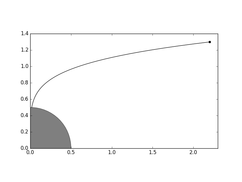
Fig. 5.2 With $A=\mathbf{Diag}(-0.3,-0.06)$ and starting point $x(0)=(2.2,1.3)$ the trajectory reaches distance $\epsilon =0.5$ from origin at time $t\approx 15.936$.

5.4.4 Logistic regression

Logistic regression is a technique of training a binary classifier. We are given a training set of examples $x_1,\dots ,x_n\in {\mathbb{R}}^d$ together with labels $y_i\in \{0,1\}$. The goal is to train a classifier capable of assigning new data points to either class 0 or 1. Specifically, the labels should be assigned by computing

(5.26)$$h_{\theta }(x)=\frac{1}{1+\exp (-{\theta }^{T}x)}$$

and choosing label $y=0$ if $h_{\theta }(x)<\frac{1}{2}$ and $y=1$ for $h_{\theta }(x)\ge \frac{1}{2}$. Here $h_{\theta }(x)$ is interpreted as the probability that $x$ belongs to class 1. The optimal parameter vector $\theta$ should be learned from the training set, so as to maximize the likelihood function:

$$\prod _i{h}_{\theta }(x_i{)}^{y_i}(1-h_{\theta }(x_i){)}^{1-y_i}.$$

By taking logarithms and adding regularization with respect to $\theta$ we reach an unconstrained optimization problem

(5.27)$${\text{minimize}}_{\theta \in {\mathbb{R}}^d}\lambda \Vert \theta {\Vert }_2+\sum _i-y_i\log (h_{\theta }(x_i))-(1-y_i)\log (1-h_{\theta }(x_i)).$$

Problem (5.27) is convex, and can be more explicitly written as

$$\begin{array}{r}\begin{array}{lrlll}\text{minimize}& \sum _i{t}_i+\lambda r& & & \\ \text{subject to}& t_i& \ge -\log (h_{\theta }(x))& =\log (1+\exp (-{\theta }^T{x}_i))& \mathrm{if}{y}_i=1,\\ & t_i& \ge -\log (1-h_{\theta }(x))& =\log (1+\exp ({\theta }^T{x}_i))& \mathrm{if}{y}_i=0,\\ & r& \ge \Vert \theta {\Vert }_2,& & \end{array}\end{array}$$

involving softplus type constraints (see Sec. 5.2 (Modeling with the exponential cone)) and a quadratic cone. See Fig. 5.3 for an example.

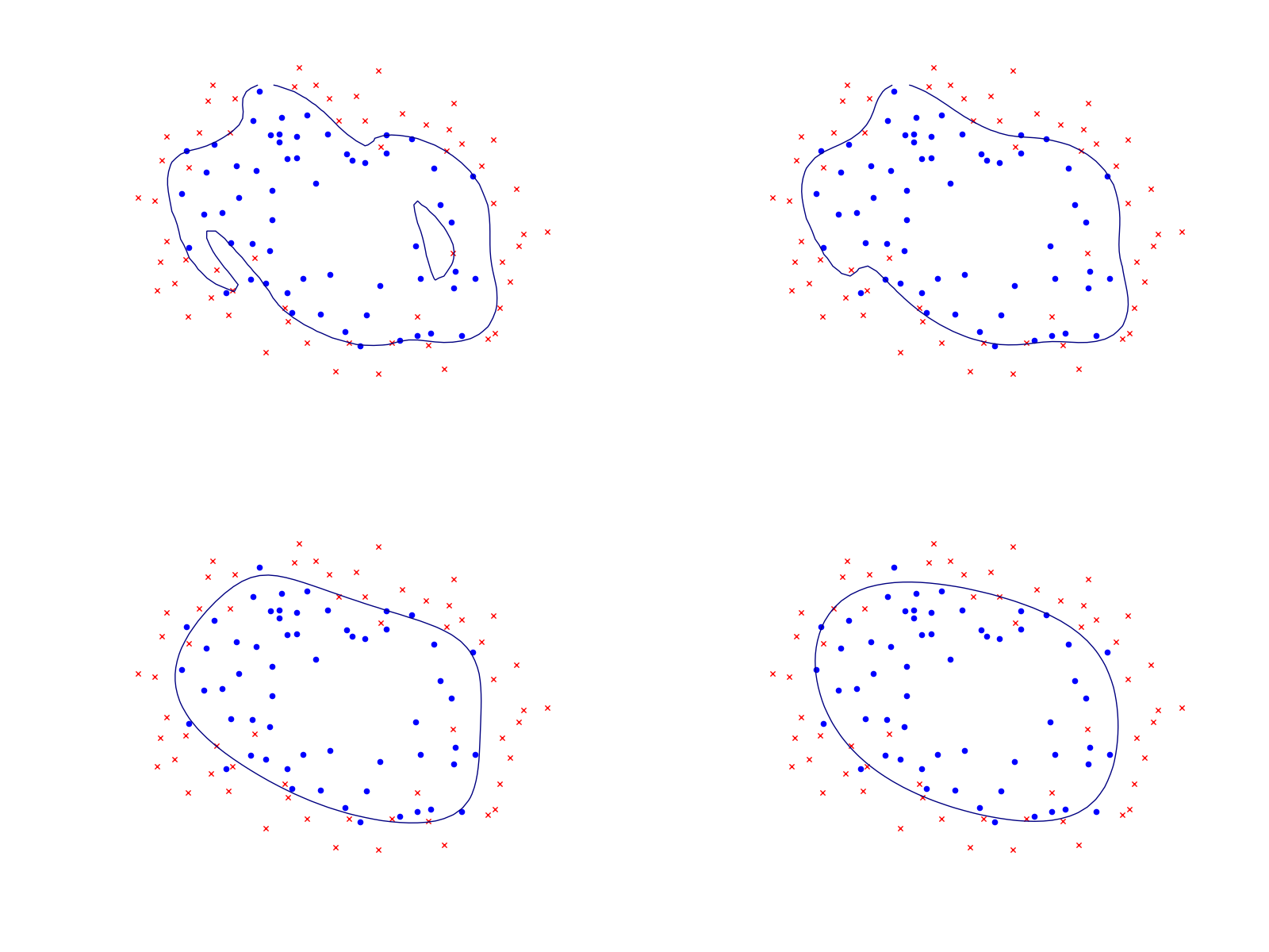
Fig. 5.3 Logistic regression example with none, medium and strong regularization (small, medium, large $\lambda$). The two-dimensional dataset was converted into a feature vector $x\in {\mathbb{R}}^{28}$ using monomial coordinates of degrees at most 6. Without regularization we get obvious overfitting.