13.4 The Optimizer for Mixed-Integer Problems

Solving optimization problems where one or more of the variables are constrained to be integer valued is called Mixed-Integer Optimization (MIO). For an introduction to model building with integer variables, the reader is recommended to consult the MOSEK Modeling Cookbook, and for further reading we highlight textbooks such as [Wol98] or [CCornuejolsZ14].

MOSEK can perform mixed-integer

• linear (MILO),

• quadratic (MIQO) and quadratically constrained (MIQCQO), and

• conic (MICO)

optimization, except for mixed-integer semidefinite problems.

By default the mixed-integer optimizer is run-to-run deterministic. This means that if a problem is solved twice on the same computer with identical parameter settings and no time limit, then the obtained solutions will be identical. The mixed-integer optimizer is parallelized, i.e., it can exploit multiple cores during the optimization.

In practice, a predominant special case of integer variables are binary variables, taking values in \(\{0,1\}\). Mixed- or pure binary problems are important subclasses of mixed-integer optimization where all integer variables are of this type. In the general setting however, an integer variable may have arbitrary lower and upper bounds.

13.4.1 Branch-and-Bound

In order to succeed in solving mixed-integer problems, it can be useful to have a basic understanding of the underlying solution algorithms. The most important concept in this regard is arguably the so-called Branch-and-Bound algorithm, employed also by MOSEK. In order to comprehend Branch-and-Bound, the concept of a relaxation is important.

Consider for example a mixed-integer linear optimization problem of minimization type

(13.12)\[\begin{split}\begin{array}{rccccl} z^* & = & \mbox{minimize} & c^T x & & \\ & & \mbox{subject to} & A x & = & b \\ & & & x \geq 0 & & \\ & & & x_j \in \integral, & & \forall j \in \mathcal{J}. \end{array}\end{split}\]

It has the continuous relaxation

(13.13)\[\begin{split}\begin{array}{rclcccl} \underline{z} & = & \mbox{minimize} & c^T x & & \\ & & \mbox{subject to} & A x & = & b\\ & & & x \geq 0, & & \end{array}\end{split}\]

obtained simply by ignoring the integrality restrictions. The first step in Branch-and-Bound is to solve this so-called root relaxation, which is a continuous optimization problem. Since (13.13) is less constrained than (13.12), one certainly gets

\[\underline{z}\leq z^*,\]

and \(\underline{z}\) is therefore called the objective bound: it bounds the optimal objective value from below.

After the solution of the root relaxation, in the most likely outcome there will be one or more integer constrained variables with fractional values, i.e., violating the integrality constraints. Branch-and-Bound now takes such a variable, \(x_j = f_j\in\mathbb{R}\setminus\mathbb{Z}\) with \(j\in\mathcal{J}\), say, and creates two branches leading to relaxations with the additional constraint \(x_j \leq \lfloor f_j \rfloor\) or \(x_j \geq \lceil f_j \rceil\), respectively. The intuitive idea here is to push the variable away from the fractional value, closer towards integrality. If the variable was binary, say, branching would lead to fixing its value to \(0\) in one branch, and to \(1\) in the other.

The Branch-and-Bound process continues in this way and successively solves relaxations and creates branches to refined relaxations. Whenever a relaxation solution \(\hat{x}\) does not violate any integrality constraints, it is feasible to (13.12) and is called an integer feasible solution. Clearly, its solution value \(\bar{z} := c^T \hat{x}\) is an upper bound on the optimal objective value,

\[z^* \leq \bar{z}.\]

Since refining a relaxation by adding constraints to it can only increase its solution value, the objective bound \(\underline{z}\), now defined as the minimum over all solution values of so far solved relaxations, can only increase during the algorithm. If as upper bound \(\bar{z}\) one records the solution value of the best integer feasible solution encountered so far, the so-called incumbent solution, \(\bar{z}\) can only decrease during the algorithm. Since at any time we also have

\[\underline{z} \leq z^* \leq \bar{z},\]

objective bound and incumbent solution value are encapsulating the optimal objective value, eventually converging to it.

The Branch-and-Bound scheme can be depicted by means of a tree, where branches and relaxations correspond to edges and nodes. Figure Fig. 13.1 shows an example of such a tree. The strength of Branch-and-Bound is its ability to prune nodes in this tree, meaning that no new child nodes will be created. Pruning can occur in several cases:

• A relaxation leads to an integer feasible solution \(\hat{x}\). In this case we may update the incumbent and its solution value \(\bar{z}\), but no new branches need to be created.

• A relaxation is infeasible. The subtree rooted at this node cannot contain any feasible relaxation, so it can be discarded.

• A relaxation has a solution value that exceeds \(\bar{z}\). The subtree rooted at this node cannot contain any integer feasible solution with a solution value better than the incumbent we already have, so it can be discarded.

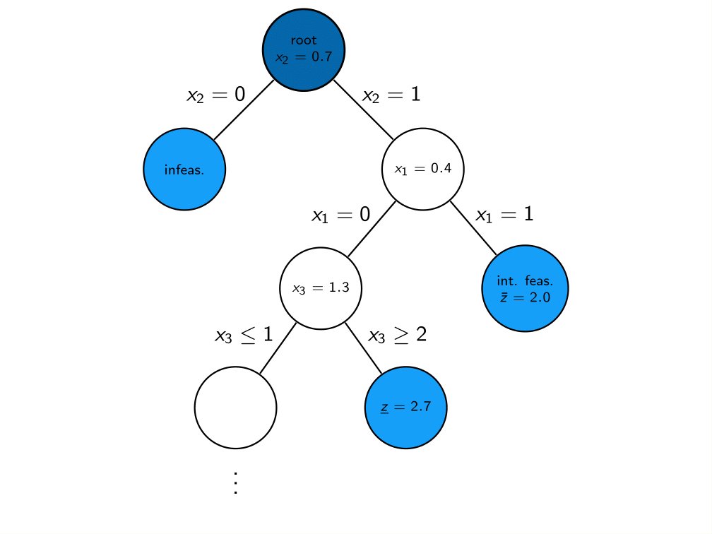
Fig. 13.1 An examplary Branch-and-Bound tree. Pruned nodes are shown in light blue.

Having objective bound and incumbent solution value is a quite fundamental property of Branch-and-Bound, and helps to asses solution quality and control termination of the algorithm, as we detail in the next section. Note that the above explanation is coined for minimization problems, but the Branch-and-bound scheme has a straightforward extension to maximization problems.

13.4.2 Solution quality and termination criteria

The issue of terminating the mixed-integer optimizer is rather delicate. Recalling the Branch-and-Bound scheme from the previous section, one may see that mixed-integer optimization is generally much harder than continuous optimization; in fact, solving continuous sub-problems is just one component of a mixed-integer optimizer. Despite the ability to prune nodes in the tree, the computational effort required to solve mixed-integer problems grows exponentially with the size of the problem in a worst-case scenario (solving mixed-integer problems is NP-hard). For instance, a problem with \(n\) binary variables, may require the solution of \(2^n\) relaxations. The value of \(2^n\) is huge even for moderate values of \(n\). In practice it is often advisable to accept near-optimal or appproximate solutions in order to counteract this complexity burden. The user has numerous possibilities of influencing optimizer termination with various parameters, in particular related to solution quality, and the most important ones are highlighted here.

13.4.2.1 Solution quality in terms of optimality

In order to assess the quality of any incumbent solution in terms of its objective value, one may check the optimality gap, defined as

\[\epsilon= |\mbox{(incumbent solution value)}-\mbox{(objective bound)}| = |\bar{z}-\underline{z}|.\]

It measures how much the objectives of the incumbent and the optimal solution can deviate in the worst case. Often it is more meaningful to look at the relative optimality gap

\[\epsilon_{\textrm{rel}} = \frac{|\bar{z}-\underline{z}|}{\max(\delta_1, |\bar{z}|)}.\]

This is essentially the above absolute optimality gap normalized against the magnitude of the incumbent solution value; the purpose of the (small) constant \(\delta_1\) is to avoid overweighing incumbent solution values that are very close to zero. The relative optimality gap can thus be interpreted as answering the question: “Within what fraction of the optimal solution is the incumbent solution in the worst case?”

Absolute and relative optimality gaps provide useful means to define termination criteria for the mixed-integer optimizer in MOSEK. The idea is to terminate the optimization process as soon as the quality of the incumbent solution, measured in absolute or relative gap, is good enough. In fact, whenever an incumbent solution is located, the criterion

\[\bar{z} - \underline{z} \leq \max (\delta_2, \delta_3 \max (\delta_1,|\bar{z}|))\]

is checked. If satisfied, i.e., if either absolute or relative optimality gap are below the thresholds \(\delta_2\) or \(\delta_3\), respectively, the optimizer terminates and reports the incumbent as an optimal solution. The optimality gaps can always be retrieved through the information items dinfitem.mio_obj_abs_gap and dinfitem.mio_obj_rel_gap.

The tolerances discussed above can be adjusted using suitable parameters, see Table 13.3. By default, the optimality parameters \(\delta_2\) and \(\delta_3\) are quite small, i.e., restrictive. These default values for the absolute and relative gap amount to solving any instance to (almost) optimality: the incumbent is required to be within at most a tiny percentage of the optimal solution. As anticipated, this is not tractable in most practical situations, and one should resort to finding near-optimal solutions quickly rather than insisting on finding the optimal one. It may happen, for example, that an optimal or close-to-optimal solution is found very early by the optimizer, but it does not terminate because the objective bound \(\underline{z}\) is of poor quality. Instead, the vast majority of computational time is spent on trying to improve \(\underline{z}\): a typical situation that practioneers would want to avoid. The concept of optimality gaps is fundamental for controlling solution quality when resorting to near-optimal solutions.

MIO performance tweaks: termination criteria

One of the first things to do in order to cut down excessive solution time is to increase the relative gap tolerance dparam.mio_tol_rel_gap to some non-default value, so as to not insist on finding optimal solutions. Typical values could be \(0.01, 0.05\) or \(0.1\), guaranteeing that the delivered solutions lie within \(1\%, 5\%\) or \(10\%\) of the optimum. Increasing the tolerance will lead to less computational time spent by the optimizer.

13.4.2.2 Solution quality in terms of feasibility

For an optimizer relying on floating-point arithmetic like the mixed-integer optimizer in MOSEK, it may be hard to achieve exact integrality of the solution values of integer variables in most cases, and it makes sense to numerically relax this constraint. Any candidate solution \(\hat{x}\) is accepted as integer feasible if the criterion

\[\min (\hat{x_j}-\lfloor \hat{x_j} \rfloor,\lceil \hat{x_j} \rceil - \hat{x_j}) \leq \delta_4 \quad \forall j \in \mathcal{J}\]

is satisfied, meaning that \(\hat{x_j}\) is at most \(\delta_4\) away from the nearest integer. As above, \(\delta_4\) can be adjusted using a parameter, see Table 13.3, and impacts the quality of the acieved solution in terms of integer feasibility. By influencing what solution may be accepted as imcumbent, it can also have an impact on the termination of the optimizer.

MIO performance tweaks: feasibility criteria

Whether increasing the integer feasibility tolerance dparam.mio_tol_abs_relax_int leads to less solution time is highly problem dependent. Intuitively, the optimizer is more flexible in finding new incumbent soutions so as to improve \(\bar{z}\). But this effect has do be examined with care on indivuidual instances: it may worsen solution quality with no effect at all on the solution time. It may in some cases even lead to contrary effects on the solution time.

Table 13.3 Tolerances for the mixed-integer optimizer.

Tolerance	Parameter name	Default value
\(\delta_1\)	dparam.mio_rel_gap_const	1.0e-10
\(\delta_2\)	dparam.mio_tol_abs_gap	0.0
\(\delta_3\)	dparam.mio_tol_rel_gap	1.0e-4
\(\delta_4\)	dparam.mio_tol_abs_relax_int	1.0e-5

13.4.2.3 Further controlling optimizer termination

There are more ways to limit the computational effort employed by the mixed-integer optimizer by simply limiting the number of explored branches, solved relaxations or updates of the incumbent solution. When any of the imposed limits is hit, the optimizer terminates and the incumbent solution may be retrieved. See Table 13.4 for a list of corresponding parameters. In contrast to the parameters discussed in Sec. 13.4.2.1 (Solution quality in terms of optimality), interfering with these does not maintain any guarantees in terms of solution quality.

Table 13.4 Other parameters affecting the integer optimizer termination criterion.

Parameter name	Explanation
iparam.mio_max_num_branches	Maximum number of branches allowed.
iparam.mio_max_num_relaxs	Maximum number of relaxations allowed.
iparam.mio_max_num_solutions	Maximum number of feasible integer solutions allowed.

13.4.3 Additional components of the mixed-integer Optimizer

The Branch-and-Bound scheme from Sec. 13.4.1 (Branch-and-Bound) is only the basic skeleton of the mixed-integer optimizer in MOSEK, and several components are built on top of that in order to enhance its functionality and increase its speed. A mixed-integer optimizer is sometimes referred to as a “giant bag of tricks”, and it would be impossible to describe all of these tricks here. Yet, some of the additional components are worth mentioning to the user. They can be influenced by various user parameters, and although the default values of these parameters are optimized to work well on average mixed-integer problems, it may pay off to adjust them for an individual problem, or a specific problem class.

13.4.3.1 Presolve

Similar to the case of continuous problems, see Sec. 13.1 (Presolve), the mixed-integer optimizer applies various presolve reductions before the actual solution process is initiated. Just as in the continuous case, the use of presolve can be controlled with the parameter iparam.presolve_use.

13.4.3.2 Primal Heuristics

Solving relaxations in the Branch-and-bound tree to an integer feasible solution \(\hat{x}\) is not the only way to find new incumbent solutions. There is a variety of procedures that, given a mixed-integer problem in a generic form like (13.12), attempt to produce integer feasible solutions in an ad-hoc way. These procedures are called Primal Heuristics, and several of them are implemented in MOSEK. For example, whenever a relaxation leads to a fractional solution, one may round the solution values of the integer variables, in various ways, and hope that the outcome is still feasible to the remaining constraints. Primal heuristics are mostly employed while processing the root node, but play a role throughout the whole solution process. The goal of a primal heuristic is to improve the incumbent solution and thus the bound \(\bar{z}\), and this can of course affect the quality of the solution that is returned after termination of the optimizer. The user parameters affecting primal heuristics are listed in Table 13.5.

MIO performance tweaks: primal heuristics

• If the mixed-integer optimizer struggles to improve the incumbent solution \(\bar{z}\), see Sec. 13.4.4 (The Mixed-Integer Log), it can be helpful to intensify the use of primal heuristics.

  • Set parameters related to primal heuristics to more aggressive values than the default ones, so that more effort is spent in this component. A List of the respective parameters can be found in Table 13.5. In particular, if the optimizer has difficulties finding any integer feasible solution at all, indicated by NA in the column BEST_INT_OBJ in the mixed-integer log, one may try to activate a construction heuristic like the Feasibility Pump with iparam.mio_feaspump_level.

  • Specify a good initial solution: In many cases a good feasible solution is either known or easily computed using problem-specific knowledge that the optimizer does not have. If so, it is usually worthwhile to use this as a starting point for the mixed-integer optimizer. See Sec. 6.8.2 (Specifying an initial solution).

  • For feasibility problems, i.e., problems having a constant objective, the goal is to find a single integer feasible solution, and this can be hard by itself on some instances. Try setting the objective to something meaningful anyway, even if the underlying application does not require this. After all, the feasible set is not changed, but the optimizer might benefit from being able to pursue a concrete goal.

• In rare cases it may also happen that the optimizer spends an excessive amount of time on primal heuristics without drawing any benefit from it, and one may try to limit their use with the respective parameters.

Table 13.5 Parameters affecting primal heuristics

Parameter name	Explanation
iparam.mio_heuristic_level	Primal heuristics aggressivity level.
iparam.mio_rins_max_nodes	Maximum number of nodes allowed in the RINS heuristic.
iparam.mio_feaspump_level	Way of using the Feasibility Pump heuristic.

13.4.3.3 Cutting Planes

Cutting planes (cuts) are simply constraints that are valid for a mixed-integer problem, for example in the form (13.12), meaning they do not remove any integer feasible solutions from the feasible set. Therefore they are also called valid inequalities. They do not have to be valid for the relaxation (13.13) though, and of interest and potentially useful are those cuts that do remove solutions from the feasible set of the relaxation. The latter is a superset of the feasible region of the mixed-integer problem, and the rationale behind cuts is thus to bring the integer problem and its relaxation closer together in terms of their feasible sets.

As an example, take the constraints

(13.14)\[2x_1 + 3x_2 + x_3 \leq 4,\quad x_1,x_2\in\{0,1\},\quad x_3\geq 0.\]

One may realize that there cannot be a feasible solution in which both binary variables take on a value of \(1\). So certainly

(13.15)\[x_1 + x_2 \leq 1\]

is a valid inequality. In fact, there is no integer solution satisfying (13.14), but violating (13.15). The latter does cut off a portion of the feasible region of the continuous relaxation of (13.14) though, obtained by replacing \(x_1,x_2\in\{0,1\}\) with \(x_1,x_2\in[0,1]\). For example, the fractional point \((x_1, x_2, x_3) = (0.5, 1, 0)\) is feasible to the relaxation, but violates the cut (13.15).

There are many classes of general-purpose cuttting planes that may be generated for a mixed-integer problem in a generic form like (13.12), and MOSEK’s mixed-integer optimizer supports several of them. For instance, the above is an example of a so-called clique cut. The most effort on generating cutting planes is spent after the solution of the root relaxation, but cuts can also be generated later on in the Branch-and-Bound tree. Cuts aim at improving the objective bound \(\underline{z}\) and can thus have significant impact on the solution time. The user parameters affecting cut generation can be seen in Table 13.6.

MIO performance tweaks: cutting planes

• If the mixed-integer optimizer struggles to improve the objective bound \(\underline{z}\), see Sec. 13.4.4 (The Mixed-Integer Log), it can be helpful to intensify the use of cutting planes.

  • Some types of cutting planes are not activated by default, but doing so may help to improve the objective bound.

  • The parameters dparam.mio_tol_rel_dual_bound_improvement and iparam.mio_cut_selection_level determine how aggressively cuts will be generated and selected.

  • If some valid inequalities can be deduced from problem-specific knowledge that the optimizer does not have, it may be helpful to add these to the problem formulation as constraints. This has to be done with care, since there is a tradeoff between the benefit obtained from an improved objective boud, and the amount of additional constraints that make the relaxations larger.

• In rare cases it may also be observed that the optimizer spends an excessive amount of time on cutting planes, see Sec. 13.4.4 (The Mixed-Integer Log), and one may limit their use with iparam.mio_max_num_root_cut_rounds, or by disabling a certain type of cutting planes.

Table 13.6 Parameters affecting cutting planes

Parameter name	Explanation
iparam.mio_cut_clique	Should clique cuts be enabled?
iparam.mio_cut_cmir	Should mixed-integer rounding cuts be enabled?
iparam.mio_cut_gmi	Should GMI cuts be enabled?
iparam.mio_cut_implied_bound	Should implied bound cuts be enabled?
iparam.mio_cut_knapsack_cover	Should knapsack cover cuts be enabled?
iparam.mio_cut_lipro	Should lift-and-project cuts be enabled?
iparam.mio_cut_selection_level	Cut selection aggressivity level.
iparam.mio_max_num_root_cut_rounds	Maximum number of root cut rounds.
dparam.mio_tol_rel_dual_bound_improvement	Minimum required objective bound improvement during root cut generation.

13.4.4 The Mixed-Integer Log

Below is a typical log output from the mixed-integer optimizer:

Presolved problem: 1176 variables, 1344 constraints, 4968 non-zeros
Presolved problem: 328 general integer, 392 binary, 456 continuous
Clique table size: 55
BRANCHES RELAXS   ACT_NDS  DEPTH    BEST_INT_OBJ         BEST_RELAX_OBJ       REL_GAP(%)  TIME
0        0        1        0        8.3888091139e+07     NA                   NA          0.0
0        1        1        0        8.3888091139e+07     2.5492512136e+07     69.61       0.1
0        1        1        0        3.1273162420e+07     2.5492512136e+07     18.48       0.1
0        1        1        0        2.6047699632e+07     2.5492512136e+07     2.13        0.2
Cut generation started.
0        1        1        0        2.6047699632e+07     2.5492512136e+07     2.13        0.2
0        2        1        0        2.6047699632e+07     2.5589986247e+07     1.76        0.2
Cut generation terminated. Time = 0.05
0        4        1        0        2.5990071367e+07     2.5662741991e+07     1.26        0.3
0        8        1        0        2.5971002767e+07     2.5662741991e+07     1.19        0.5
0        11       1        0        2.5925040617e+07     2.5662741991e+07     1.01        0.5
0        12       1        0        2.5915504014e+07     2.5662741991e+07     0.98        0.5
2        23       1        0        2.5915504014e+07     2.5662741991e+07     0.98        0.6
14       35       1        0        2.5915504014e+07     2.5662741991e+07     0.98        0.6

[ ... ]

Objective of best integer solution : 2.578282162804e+07
Best objective bound               : 2.569877601306e+07
Construct solution objective       : Not employed
User objective cut value           : Not employed
Number of cuts generated           : 192
  Number of Gomory cuts            : 52
  Number of CMIR cuts              : 137
  Number of clique cuts            : 3
Number of branches                 : 29252
Number of relaxations solved       : 31280
Number of interior point iterations: 16
Number of simplex iterations       : 105440
Time spend presolving the root     : 0.03
Time spend optimizing the root     : 0.07
Mixed integer optimizer terminated. Time: 6.46

The first lines contain a summary of the problem after mixed-integer presolve has been applied. This is followed by the iteration log, reflecting the progress made during the Branch-and-bound process. The columns have the following meanings:

• BRANCHES: Number of branches / nodes generated.

• RELAXS: Number of relaxations solved.

• ACT_NDS: Number of active / non-processed nodes.

• DEPTH: Depth of the last solved node.

• BEST_INT_OBJ: The incumbent solution / best integer objective value, \(\bar{z}\).

• BEST_RELAX_OBJ: The objective bound, \(\underline{z}\).

• REL_GAP(%): Relative optimality gap, \(100\%\cdot\epsilon_{\textrm{rel}}\)

• TIME: Time (in seconds) from the start of optimization.

The beginning and the end of the root cut generation is highlighted as well, and the number of log lines in between reflects to the computational effort spent here.

Finally there is a summary of the optimization process, containing also information on the type of generated cuts and the total number of iterations needed to solve all occuring continuous relaxations.

When the solution time for a mixed-integer problem has to be cut down, it can sometimes be useful to examine the log in order to understand where time is spent and what might be improved. In particular, it might happen that the values in either of the colums BEST_INT_OBJ or BEST_RELAX_OBJ stall over a long period of log lines, an indication that the optimizer has a hard time improving either the incumbent solution, i.e., \(\bar{z}\), or the objective bound \(\underline{z}\), see also Sec. 13.4.3.2 (Primal Heuristics) and Sec. 13.4.3.3 (Cutting Planes).

13.4.5 Mixed-Integer Nonlinear Optimization

Due to the involved non-linearities, MI(QC)QO or MICO problems are on average harder than MILO problems of comparable size. Yet, the Branch-and-Bound scheme can be applied to these probelm classes in a straightforward manner. The relaxations have to be solved as conic problems with the interior point algorithm in that case, see Sec. 13.3 (Conic Optimization - Interior-point optimizer), opposed to MILO where it is often beneficial to solve relaxations with the dual simplex method, see Sec. 13.2.3 (The Simplex Optimizer). There is another solution approach for these types of problems implemented in MOSEK, namely the Outer-Approximation algorithm, making use of dynamically refined linear approximations of the non-linearities.

MICO performance tweaks: choice of algorithm

Whether conic Branch-and-Bound or Outer-Approximation is applied to a mixed-integer conic problem can be set with iparam.mio_conic_outer_approximation. The best value for this option is highly problem dependent.

13.4.5.1 MI(QC)QO

MOSEK is specialized in solving linear and conic optimization problems, both with or without mixed-integer variables. Just like for continuous problems, mixed-integer quadratic problems are converted internally to conic form, see Sec. 12.4.1 (A Recommendation)

Contrary to the continuous case, MOSEK can solve certain mixed-integer quadratic problems where one or more of the involved matrices are not positive semidefinite, so-called non-convex MI(QC)QO problems. These are automatically reformulated to an equivalent convex MI(QC)QO problem, provided that such a reformulation is possible on the given instance (otherwiese MOSEK will reject the problem and issue an error message). The concept of reformulations can also affect the solution times of MI(QC)QO problems.

MI(QC)QO performance tweaks: applying a reformulation method

There are several reformulation methods for MI(QC)QO problems, available through the parameter iparam.mio_qcqo_reformulation_method. The chosen method can have significant impact on the mixed-integer optimizer’s speed on such problems, both convex and non-convex. The best value for this option is highly problem dependent.

13.4.6 Disjunctive constraints

Problems with disjunctive constraints (DJC) see Sec. 6.9 (Disjunctive constraints) are typically reformulated to mixed-integer problems, and even if this is not the case they are solved with an algorithm that is based on the mixed-integer optimizer. In MOSEK, these problems thus fall into the realm of MIO. In particular, MOSEK automatically attempts to replace any DJC by so called big-M constraints, potentially after transforming it to several, less complicated DJCs. As an example, take the DJC

\[[z = 0] \vee [z = 1, x_1 + x_2 \geq 1000],\]

where \(z\in\{0,1\}\) and \(x_1, x_2 \in [0,750]\). This is an example of a DJC formulation of a so-called indicator constraint. A big-M reformulation is given by

\[x_1 + x_2 \geq 1000 - M \cdot (1 - z),\]

where \(M > 0\) is a large constant. The practical difficulty of these constructs is that \(M\) should always be sufficiently large, but ideally not larger. Too large values for \(M\) can be harmful for the mixed-integer optimizer. During presolve, and taking into account the bounds of the involved variables, MOSEK automatically reformulates DJCs to big-M constraints if the required \(M\) values do not exceed the parameter dparam.mio_djc_max_bigm. From a performance point-of-view, all DJCs would ideally be linearized to big-Ms after presolve without changing this parameter’s default value of 1.0e6. Whether or not this is the case can be seen by retrieving the information item iinfitem.mio_presolved_numdjc, or by a line in the mixed-integer optimizer’s log as in the example below. Both state the number of remaining disjunctions after presolve.

Presolved problem: 305 variables, 204 constraints, 708 non-zeros
Presolved problem: 0 general integer, 100 binary, 205 continuous
Presolved problem: 100 disjunctions
Clique table size: 0
BRANCHES RELAXS   ACT_NDS  DEPTH    BEST_INT_OBJ         BEST_RELAX_OBJ       REL_GAP(%)  TIME
0        1        1        0        NA                   0.0000000000e+00     NA          0.0
0        1        1        0        5.0574653969e+05     0.0000000000e+00     100.00      0.0

[ ... ]

DJC performance tweaks: managing variable bounds

• Always specify the tightest known bounds on the variables of any problem with DJCs, even if they seem trivial from the user-perspective. The mixed-integer optimizer can only benefit from these when reformulating DJCs and thus gain performance; even if bounds don’t help with reformulations, it is very unlikely that they hurt the optimizer.

• Increasing dparam.mio_djc_max_bigm can lead to more DJC reformulations and thus increase optimizer speed, but it may in turn hurt numerical solution quality and has to be examined with care. The other way round, on numerically challenging instances with DJCs, decreasing dparam.mio_djc_max_bigm may lead to numerically more robust solutions.

13.4.7 Randomization

A mixed-integer optimizer is usually prone to performance variability, meaning that a small change in either

• problem data, or

• computer hardware, or

• algorithmic parameters

can lead to significant changes in solution time, due to different solution paths in the Branch-and-Bound tree. In extreme cases the exact same problem can vary from being solvable in less than a second to seemingly unsolvable in any reasonable amount of time on a different computer.

One practical implication of this is that one should ideally verify whether a seemingly beneficial set of parameters, established experimentally on a single problem, is still beneficial (on average) on a larger set of problems from the same problem class. This protects against making parameter changes that had positive effects only due to random effects on that single problem.

In the absence of a large set of test problems, one may also change the random seed of the optimizer to a series of different values in order to hedge against drawing such wrong conclusions regarding parameters. The random seed, accessible through iparam.mio_seed, impacts for example random tie-breaking in many of the mixed-integer optimizer’s components. Changing the random seed can be combined with a permutation of the problem data to further incite randomness, accessible through the parameter iparam.mio_data_permutation_method.

13.4.8 Further performance tweaks

In addition to what was mentioned previously, there may be other ways to speed up the solution of a given mixed-integer problem. For example, there are further user parameters affecting some algorithmic settings in the mixed-integer optimizer. As mentioned above, default parameter values are optimized to work well on average, but on individual problems they may be adjusted.

MIO performance tweaks: miscellaneous

• When relaxations in the the Branch-and-Bound tree are linear optimization problems (e.g., in MILO or when solving MICO probelms with the Outer-Approximation method), it is usually best to employ the dual simplex method for their solution. In rare cases the primal simplex method may actually be the better choice, and this can be set with the parameter iparam.mio_node_optimizer.

• Some problems are numerically more challenging than others, for example if the ratio between the smallest and the largest involved coefficients is large, say \(\geq 1e9\). An indication of numerical issues are, for example, large violations in the final solution, observable in the solution summery of the log output, see Sec. 8.1.3 (Mixed-integer problem). Similarly, a problem that is known to be feasible by the user may be declared infeasible by the optimizer. In such cases it is usually best to try to rescale the model. Otherwise, the mixed-integer optimizer can be instructed to be more cautios regarding numerics with the parameter iparam.mio_numerical_emphasis_level. This may in turn be at the cost of solution speed though.

• Improve the formulation: A MIO problem may be impossible to solve in one form and quite easy in another form. However, it is beyond the scope of this manual to discuss good formulations for mixed-integer problems. For discussions on this topic see for example [Wol98].