6 Conic Modeling

6.1 The model

A model built using Fusion is always a conic optimization problem and it is convex by definition. These problems can be succinctly characterized as

(6.1)$$\begin{array}{r}\begin{array}{lll}\text{minimize}& c^{T}x& \\ \text{subject to}& Ax+b\in \mathcal{K}& \end{array}\end{array}$$

where $\mathcal{K}$ is a product of domains supported by MOSEK, in particular:

• linear: $\mathbb{R}$, ${\mathbb{R}}_{+}$, $\{0\}$,

• quadratic: ${\mathcal{Q}}^n=\{x\in {\mathbb{R}}^n:x_1\ge \sqrt{x_2^2+\cdots +x_n^2}\}$,

• rotated quadratic: ${\mathcal{Q}}_r^n=\{x\in {\mathbb{R}}^n:2x_1{x}_2\ge x_3^2+\cdots +x_n^2,x_1,x_2\ge 0\}$,

• primal power cone: ${\mathcal{P}}_n^{\alpha ,1-\alpha }=\{x\in {\mathbb{R}}^n:x_1^{\alpha }{x}_2^{1-\alpha }\ge \sqrt{x_3^2+\cdots +x_n^2},x_1,x_2\ge 0\}$, or its dual,

• primal exponential: $K_{\exp }=\{x\in {\mathbb{R}}^3:x_1\ge x_2\exp (x_3/x_2),x_1,x_2\ge 0\}$, or its dual,

• semidefinite:: ${\mathcal{S}}_{+}^n=\{X\in {\mathbb{R}}^{n\times n}:X\text{is symmetric positive semidefinite}\}$.

• and others, see Sec. 14.9 (Supported domains) for a full list.

The main thing about a Fusion model is that it can be specified in a convenient way without explicitly constructing the representation (6.1). Instead the user has access to variables which are used to construct linear operators that appear in constraints. The cone types described above are the domains of those constraints. A Fusion model can potentially contain many different building blocks of that kind. To facilitate manipulations with a large number of variables Fusion defines various logical views of parts of the model. To facilitate reoptimizing the same problem with varying input data Fusion provides parameters.

This section briefly summarizes the constructions and techniques available in Fusion. See Sec. 7 (Optimization Tutorials) for a basic tutorial and Sec. 11 (Case Studies) for more advanced case studies. This section is only an introduction: detailed specification of the methods and classes mentioned here can be found in the API reference.

A Fusion model is represented by the class Model and created by a simple construction

M = Model()
M = Model('modelName')

with Model() as M:

The model object is the user’s interface to the optimization problem, used in particular for

• formulating the problem by defining variables, parameters, constraints and objective,

• solving the problem and retrieving the solution status and solutions,

• interacting with the solver: setting up parameters, registering for callbacks, performing I/O, obtaining detailed information from the optimizer etc.

Almost all elements of the model: variables, parameters, constraints and the model itself can be constructed with or without names. If used, the names for each type of object must be unique. Choosing a good naming convention can make the problem more readable when dumped to a file.

6.2 Variables

Continuous variables can be scalars, vectors or higher-dimensional arrays. The are added to the model with the method Model.variable which returns a representing object of type Variable. The shape of a variable (number of dimensions and length in each dimension) has to be specified at creation. Optionally a variable may be created in a restricted domain (by default variables are unbounded, that is in $\mathbb{R}$). For instance, to declare a variable $x\in {\mathbb{R}}_{+}^n$ we could write

    x = M.variable("x", n, Domain.greaterThan(0.))

A multi-dimensional variable is declared by specifying an array with all dimension sizes. Here is an $n\times n$ variable:

    x = M.variable( [n,n], Domain.unbounded() ) 

The specification of dimensions can also be part of the domain, as in this declaration of a symmetric positive semidefinite variable of dimension $n$:

    v = M.variable(Domain.inPSDCone(n));

Integer variables are specified with an additional domain modifier. To add an integer variable $z\in [1,10]$ we write

    z= M.variable('z', Domain.integral(Domain.inRange(1.,10.)) )

The function Domain.binary is a shorthand for binary variables often appearing in combinatorial problems:

    y= M.variable('y', Domain.binary())

Integrality requirement can be switched on and off using the methods Variable.makeInteger and Variable.makeContinuous.

A domain usually allows to specify the number of objects to be created. For example here is a definition of $m$ symmetric positive semidefinite variables of dimension $n$ each. The actual variable x will be of shape $m\times n\times n$ where each slice with fixed first coordinate is an $n\times n$ PSD:

    x = M.variable(Domain.inPSDCone(n, m))

The Variable object provides the primal (Variable.level) and dual (Variable.dual) solution values of the variable after optimization, and it enters in the construction of linear expressions involving the variable.

6.3 Expressions and linear operators

Linear expressions are constructed combining variables, parameters, matrices and other constant values by linear operators. The result is an object that represents the linear expression itself. Fusion only allows for those combinations of operators and arguments that yield linear functions of the variables. Expressions have shapes and dimensions in the same fashion as variables. For instance, if $x\in {\mathbb{R}}^n$ and $A\in {\mathbb{R}}^{m\times n}$, then $Ax$ is a vector expression of length $m$. Note, however, that the internal size of $Ax$ is $mn$, because each entry is a linear combination for which $m$ coefficients have to be stored.

Expressions are concrete implementations of the virtual interface Expression. In typical situations, however, all operations on expressions can be performed using the static methods and factory methods of the class Expr.

Table 6.1 Linear Operators

Method	Description
Expr.add (+)	Element-wise addition of two matrices
Expr.sub (-)	Element-wise subtraction of two matrices
Expr.mul (*,@)	Matrix or matrix-scalar multiplication
Expr.neg (-)	Sign inversion
Expr.outer	Vector outer-product
Expr.dot	Dot product
Expr.sum	Sum over a given dimension
Expr.mulElm	Element-wise multiplication
Expr.mulDiag	Sum over the diagonal of a matrix which is the result of a matrix multiplication
Expr.constTerm	Return a constant term

Operations on expressions must adhere to the rules of matrix algebra regarding dimensions; otherwise a DimensionError exception will be thrown.

Expression can be composed, nested and used as building blocks in new expressions. For instance $Ax+By$ can be implemented as:

    Expr.add( Expr.mul(A,x), Expr.mul(B,y) )

For operations involving multiple variables and expressions the users should consider list-based methods. For instance, a clean way to write $x+y+z+w$ would be:

    Expr.add( [x, y, z, w] )

Note that a single variable (object of class Variable) can also be used as an expression. Once constructed, expressions are immutable.

6.4 Constraints and objective

Constraints are declared within an optimization model using the method Model.constraint. Every constraint in Fusion has the form

Expression belongs to a Domain.

Objects of type Domain correspond roughly to the types of convex cones $\mathcal{K}$ mentioned at the beginning of this section. For instance, the following set of linear constraints

(6.2)$$\begin{array}{r}\begin{array}{lccccr}{x}_1& +& 2x_2& & & =0\\ & +& x_2& +& x_3& =0\\ x_1& & & & & =0\end{array}\end{array}$$

could be declared as

    A = [ [1.0, 2.0, 0.0],
          [0.0, 1.0, 1.0],
          [ 1.0, 0.0, 0.0] ]

    x = M.variable("x",3,Domain.unbounded())
    c = M.constraint( Expr.mul(A,x), Domain.equalsTo(0.0))

Note that the scalar domain Domain.equalsTo (==) consisting of a single point $0$ scales up to the dimension of the expression and applies to all its elements. This allows many constraints to be comfortably expressed in a vectorized form. See also Sec. 6.8 (Vectorization).

The Constraint object provides the dual (Constraint.dual) value of the constraint after optimization and the primal value of the constraint expression (Constraint.level).

The typical domains used to specify constraints are listed below. Note that they can also be used directly at variable creation, whenever that makes sense.

	Type	Domain
Linear	equality	Domain.equalsTo (==)
	inequality $\le$	Domain.lessThan (<=)
	inequality $\ge$	Domain.greaterThan (>=)
	two-sided bound	Domain.inRange
Conic Quadratic	quadratic cone	Domain.inQCone
	rotated quadratic cone	Domain.inRotatedQCone
Other Conic	exponential cone	Domain.inPExpCone
	power cone	Domain.inPPowerCone
	geometric mean	Domain.inPGeoMeanCone
Semidefinite	PSD matrix	Domain.inPSDCone
Integral	Integers in domain D	Domain.integral(D)
	$\{0,1\}$	Domain.binary

See Sec. 14.9 (Supported domains) and the API reference for Domain for a full list.

Having discussed variables and constraints we can finish by defining the optimization objective with Model.objective. The objective function is an affine expression that evaluates to a scalar (that is, of shape $()$ or $(1)$) and the objective sense is specified by the enumeration ObjectiveSense as either minimize or maximize. The typical linear objective function $c^{T}x$ can be declared as

    M.objective( ObjectiveSense.Minimize,  Expr.dot(c,x) )

6.5 Matrices

At some point it becomes necessary to specify linear expressions such as $Ax$ where $A$ is a (large) constant data matrix. Such coefficient matrices can be represented in dense or sparse format. Dense matrices can always be represented using the standard data structures for arrays and two-dimensional arrays built into the language. Alternatively, or when sparsity can be exploited, matrices can be constructed as objects of the class Matrix. This can have some advantages: a more generic code that can be ported across platforms and can be used with both dense and sparse matrices without modifications.

Dense matrices are constructed with a variant of the static factory method Matrix.dense. The values of all entries must be specified all at once and the resulting matrix is immutable. For example the matrix

$$\begin{array}{r}A=\left[\begin{array}{cccc}1& 2& 3& 4\\ 5& 6& 7& 8\end{array}\right]\end{array}$$

can be defined with:

    A= [ [1, 2, 3, 4], [5, 6, 7, 8] ]
    Ad= Matrix.dense(A)

or from a flattened representation:

    A= [ 1, 2, 3, 4, 5, 6, 7, 8 ]
    Af= Matrix.dense(2, 4, A)

Sparse matrices are constructed with a variant of the static factory method Matrix.sparse. This is both speed- and memory-efficient when the matrix has few nonzero entries. A matrix $A$ in sparse format is given by a list of triples $(i,j,v)$, each defining one entry: $A_{i,j}=v$. The order does not matter. The entries not in the list are assumed to be $0$. For example, take the matrix

$$\begin{array}{r}A=\left[\begin{array}{cccc}1.0& 0.0& 0.0& 2.0\\ 0.0& 3.0& 0.0& 4.0\end{array}\right].\end{array}$$

Assuming we number rows and columns from $0$, the corresponding list of triplets is:

$$A=\{(0,0,1.0),(0,3,2.0),(1,1,3.0),(1,3,4.0)\}$$

The Fusion definition would be:

    rows  = [ 0, 0, 1, 1 ]
    cols  = [ 0, 3, 1, 3 ]
    values= [ 1.0, 2.0, 3.0, 4.0 ]

    m = Matrix.sparse(2, 4, rows, cols, values)

The Matrix class provides more standard constructions such as the identity matrix, a constant value matrix, block diagonal matrices etc.

6.6 Parameters

A parameter (Parameter) is a placeholder for a constant whose value should be specified before the model is optimized. Parameters can have arbitrary shapes, just like variables, and can be used in any place where using a constant, array or matrix of the same shape would be suitable. That means parameters behave like expressions under additive operations and stacking, and can additionally be used in some multiplicative operations where the result is affine in the optimization variables.

For example, we can create a parametrized constraint

$$p^{T}x+q\le 0,$$

where $x\in {\mathbb{R}}^4$, as follows:

    x = M.variable('x', 4)                  # Variable
    
    p = M.parameter('p', 4)                 # Parameter of shape [ 4 ]
    q = M.parameter()                       # Scalar parameter

    M.constraint(Expr.add(Expr.dot(p, x), q), Domain.lessThan(0.0))

Later in the code we can initialize the parameters with actual values. For example

    p.setValue([1,2,3,4])
    q.setValue(5)

will make the previously defined constraint evaluate to

$$x_1+2x_2+3x_3+4x_4+5\le 0.$$

The values of parameters can be changed between optimizations. Therefore one parametrized model with fixed structure can be used to solve many instances of the same optimization problem with varying input data.

6.7 Stacking and views

Fusion provides a way to construct logical views of parts of existing expressions or combinations of existing expressions. They are still represented by objects of type Variable or Expression that refer to the original ones. This can be useful in some scenarios:

• retrieving only the values of a few variables, and ignoring the remaining auxiliary ones,

• stacking vectors or matrices to perform various matrix operations,

• bundling a number of similar constraints into one; see Sec. 6.8 (Vectorization),

• adding constraints between parts of the same variable, etc.

All these operations do not require new variables or expressions, but just lightweight logical views. In what follows we will concentrate on expressions; the same techniques are available for variables. These techniques will be familiar to the users of numerical tools such as Matlab or NumPy.

Picking and slicing

Expression.pick ([]) picks a subset of entries from a variable or expression. Special cases of picking are Expression.index ([]), which picks just one scalar entry and Expression.slice ([]) which picks a slice, that is restricts each dimension to a subinterval. Slicing is a frequently used operation.

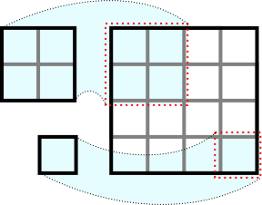
Fig. 6.1 Two dimensional slicing.

Both displayed regions are slices of the two-dimensional $4\times 4$ expression, which can be selected as follows:

    A1 = Ax.slice([0,0],[2,2])
    A2 = Ax.index([3,3])

Reshaping

Expressions can be reshaped creating a view with the same number of coordinates arranged in a different way. A particular example of this operation if flattening, which converts any multi-dimensional expression into a one-dimensional vector.

Stacking

Stacking refers to the concatenation of expressions to form a new larger one. For example, the next figure depicts the vertical stacking of two vectors of shape $1\times 3$ resulting in a matrix of shape $2\times 3$.

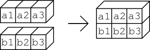
    c = Expr.vstack([a, b]);

Vertical stacking (Expr.vstack) of expressions of shapes $d_1\times d_2$ and $d_1^{\prime }\times d_2$ has shape $(d_1+d_1^{\prime })\times d_2$. Similarly, horizontal stacking (Expr.hstack) of expressions of shapes $d_1\times d_2$ and $d_1\times d_2^{\prime }$ has shape $d_1\times (d_2+d_2^{\prime })$. Fusion supports also more general versions of stacking for multi-dimensional variables, as described in Expr.stack. A special case of stacking is repetition (Expr.repeat), equivalent to stacking copies of the same expression.

6.8 Vectorization

Using Fusion one can compactly express sequences of similar constraints. For example, if we want to express

$$A{x}_i=b_i,i=1,\dots ,n$$

we can think of $x_i\in {\mathbb{R}}^m,b_i\in {\mathbb{R}}^k$ as the columns of two matrices $X=[x_1,\dots ,x_n]\in {\mathbb{R}}^{m\times n}$, $B=[b_1,\dots ,b_n]\in {\mathbb{R}}^{k\times n}$, and write simply

$$AX-B=0.$$

    X = Var.hstack( [ xi[i] for i in range(n) ] )
    B = Expr.hstack( [ bi[i] for i in range(n) ] )

    M.constraint(Expr.sub(Expr.mul(A, X), B), Domain.equalsTo(0.0))

In this example the domain Domain.equalsTo (==) scales to apply to all the entries of the expression.

Another powerful case of vectorization and scaling domains is the ability to define a sequence of conic constraints in one go. Suppose we want to find an upper bound on the 2-norm of a sequence of vectors, that is we want to express

$$t\ge \Vert y_i\Vert ,i=1,\dots ,n$$

Suppose that the vectors $y_i$ are arranged in the rows of a matrix $Y$. Then we can simply write:

    t = M.variable();

    M.constraint(Expr.hstack(Var.vrepeat(t, n), Y), Domain.inQCone())

Here, again, the conic domain Domain.inQCone is by default applied to each row of the matrix separately, yielding the desired constraints in a loop-free way (the $i$-th row is $(t,y_i)$). The direction along which conic constraints are created within multi-dimensional expressions can be changed with Domain.axis.

We recommend vectorizing the code whenever possible. It is not only more elegant and portable but also more efficient — loops are eliminated and the number of Fusion API calls is reduced.

6.9 Reoptimization

Between optimizations the user can modify the model in a few ways:

• Set/change values of parameters (Parameter.setValue). This is the recommended way to reoptimize multiple models identical structure and varying (parts of) input data. For simplicity, suppose we want to minimize $f(x)=\gamma x+\beta y$, for varying choices of $\gamma >0$. Then we could write:

  gammaValues = [0., 0.5, 1.0]                # Choices for gamma
  beta = 2.0
  with Model() as M:
      x = M.variable('x',1,Domain.greaterThan(0.))
      y = M.variable('y',1,Domain.greaterThan(0.))
      gamma = M.parameter('gamma')
      
      M.objective( ObjectiveSense.Minimize, Expr.add(Expr.mul(gamma, x), Expr.mul(beta, y)) )
  
      for g in gammaValues:     
        gamma.setValue(g)
        M.solve()
  

• Add new constraints with Model.constraint. This is useful for solving a sequence of optimization problems with more and more restrictions on the feasible set. See for example Sec. 11.8 (Travelling Salesman Problem (TSP)).

• Add new variables with Model.variable or parameters with Model.parameter.

• Replace the objective with a completely new one (Model.objective).

• Update part of the objective (Model.updateObjective).

• Update an existing constraint or replace the constraint expression with a new one (Constraint.update).

Otherwise all Fusion objects are immutable. See also Sec. 7.10 (Problem Modification and Reoptimization) for more reoptimization examples.