15.1 API Conventions

15.1.1 Function arguments

Naming Convention

In the definition of the MOSEK Optimizer API for Python a consistent naming convention has been used. This implies that whenever for example numcon is an argument in a function definition it indicates the number of constraints. In Table 15.1 the variable names used to specify the problem parameters are listed.

Table 15.1 Naming conventions used in the MOSEK Optimizer API for Python.

API name	API type	Dimension	Related problem parameter
numcon	int		\(m\)
numvar	int		\(n\)
numcone	int		\(t\)
aptrb	int[]	numvar	\(a_{ij}\)
aptre	int[]	numvar	\(a_{ij}\)
asub	int[]	aptre[numvar-1]	\(a_{ij}\)
aval	float[]	aptre[numvar-1]	\(a_{ij}\)
c	float[]	numvar	\(c_j\)
cfix	float		\(c^f\)
blc	float[]	numcon	\(l_k^c\)
buc	float[]	numcon	\(u_k^c\)
blx	float[]	numvar	\(l_k^x\)
bux	float[]	numvar	\(u_k^x\)
numqonz	int		\(q_{ij}^o\)
qosubi	int[]	numqonz	\(q_{ij}^o\)
qosubj	int[]	numqonz	\(q_{ij}^o\)
qoval	float[]	numqonz	\(q_{ij}^o\)
numqcnz	int		\(q_{ij}^k\)
qcsubk	int[]	numqcnz	\(q_{ij}^k\)
qcsubi	int[]	numqcnz	\(q_{ij}^k\)
qcsubj	int[]	numqcnz	\(q_{ij}^k\)
qcval	float[]	numqcnz	\(q_{ij}^k\)
bkc	int[]	numcon	\(l_k^c\) and \(u_k^c\)
bkx	int[]	numvar	\(l_k^x\) and \(u_k^x\)

The relation between the variable names and the problem parameters is as follows:

• The quadratic terms in the objective: \(q_{ \mathtt{qosubi[t]}, \mathtt{qosubj[t]} }^o = \mathtt{qoval[t]},\quad t=\idxbeg,\ldots ,\idxend{\mathtt{numqonz}}.\)

• The linear terms in the objective : \(c_j = \mathtt{c[j]},\quad j=\idxbeg,\ldots ,\idxend{\mathtt{numvar}}\)

• The fixed term in the objective : \(c^f = \mathtt{cfix}.\)

• The quadratic terms in the constraints: \(q_{\mathtt{qcsubi[t]},\mathtt{qcsubj[t]}}^{\mathtt{qcsubk[t]}} = \mathtt{qcval[t]},\quad t=\idxbeg,\ldots ,\idxend{\mathtt{numqcnz}}\)

• The linear terms in the constraints: \(a_{\mathtt{asub[t],j}} = \mathtt{aval[t]}, \quad t=\mathtt{ptrb[j]},\ldots ,\mathtt{ptre[j]}-1,\ j=\idxbeg,\ldots ,\idxend{\mathtt{numvar}}\)

Information about input/output arguments

The following are purely informational tags which indicate how MOSEK treats a specific function argument.

• (input) An input argument. It is used to input data to MOSEK.

• (output) An output argument. It can be a user-preallocated data structure, a reference, a string buffer etc. where MOSEK will output some data.

• (input/output) An input/output argument. MOSEK will read the data and overwrite it with new/updated information.

15.1.2 Bounds

The bounds on the constraints and variables are specified using the variables bkc, blc, and buc. The components of the integer array bkc specify the bound type according to Table 15.2

Table 15.2 Symbolic key for variable and constraint bounds.

Symbolic constant	Lower bound	Upper bound
boundkey.fx	finite	identical to the lower bound
boundkey.fr	minus infinity	plus infinity
boundkey.lo	finite	plus infinity
boundkey.ra	finite	finite
boundkey.up	minus infinity	finite

For instance bkc[2]=boundkey.lo means that \(-\infty < l_2^c\) and \(u_2^c = \infty\). Even if a variable or constraint is bounded only from below, e.g. \(x \geq 0\), both bounds are inputted or extracted; the irrelevant value is ignored.

Finally, the numerical values of the bounds are given by

\[l_k^c = \mathtt{blc[k]}, \quad k=\idxbeg,\ldots,\idxend{\mathtt{numcon}}\]

\[u_k^c = \mathtt{buc[k]}, \quad k=\idxbeg,\ldots,\idxend{\mathtt{numcon}}.\]

The bounds on the variables are specified using the variables bkx, blx, and bux in the same way. The numerical values for the lower bounds on the variables are given by

\[l_j^x = \mathtt{blx[j]}, \quad j=\idxbeg,\ldots,\idxend{\mathtt{numvar}}.\]

\[u_j^x = \mathtt{bux[j]}, \quad j=\idxbeg,\ldots,\idxend{\mathtt{numvar}}.\]

15.1.3 Vector Formats

Three different vector formats are used in the MOSEK API:

Full (dense) vector

This is simply an array where the first element corresponds to the first item, the second element to the second item etc. For example to get the linear coefficients of the objective in task with numvar variables, one would write

c = zeros(numvar,float)
task.getc(c)

Vector slice

A vector slice is a range of values from first up to and not including last entry in the vector, i.e. for the set of indices i such that first <= i < last. For example, to get the bounds associated with constrains 2 through 9 (both inclusive) one would write

upper_bound = zeros(8,float)
lower_bound = zeros(8,float)
bound_key   = array([0] * 8)

task.getconboundslice(2, 10,
                      bound_key,lower_bound,upper_bound)

Sparse vector

A sparse vector is given as an array of indexes and an array of values. The indexes need not be ordered. For example, to input a set of bounds associated with constraints number 1, 6, 3, and 9, one might write

bound_index = [          1,          6,          3,          9]
bound_key   = [boundkey.fr,boundkey.lo,boundkey.up,boundkey.fx]
lower_bound = [     0.0,         -10.0,        0.0,        5.0]
upper_bound = [     0.0,           0.0,        6.0,        5.0]
task.putconboundlist(bound_index,
                     bound_key,lower_bound,upper_bound)

15.1.4 Matrix Formats

The coefficient matrices in a problem are inputted and extracted in a sparse format. That means only the nonzero entries are listed.

15.1.4.1 Unordered Triplets

In unordered triplet format each entry is defined as a row index, a column index and a coefficient. For example, to input the \(A\) matrix coefficients for \(a_{1,2}=1.1, a_{3,3}=4.3\) , and \(a_{5,4}=0.2\) , one would write as follows:

subi = array([   1,   3,   5 ])
subj = array([   2,   3,   4 ])
cof  = array([ 1.1, 4.3, 0.2 ])
task.putaijlist(subi,subj,cof)

Please note that in some cases (like Task.putaijlist) only the specified indexes are modified — all other are unchanged. In other cases (such as Task.putqconk) the triplet format is used to modify all entries — entries that are not specified are set to \(0\).

15.1.4.2 Column or Row Ordered Sparse Matrix

In a sparse matrix format only the non-zero entries of the matrix are stored. MOSEK uses a sparse packed matrix format ordered either by columns or rows. Here we describe the column-wise format. The row-wise format is based on the same principle.

Column ordered sparse format

A sparse matrix in column ordered format is essentially a list of all non-zero entries read column by column from left to right and from top to bottom within each column. The exact representation uses four arrays:

• asub: Array of size equal to the number of nonzeros. List of row indexes.

• aval: Array of size equal to the number of nonzeros. List of non-zero entries of \(A\) ordered by columns.

• ptrb: Array of size numcol, where ptrb[j] is the position of the first value/index in aval/ asub for the \(j\)-th column.

• ptre: Array of size numcol, where ptre[j] is the position of the last value/index plus one in aval / asub for the \(j\)-th column.

With this representation the values of a matrix \(A\) with numcol columns are assigned using:

\[a_{\mathtt{asub}[k],j} = \mathtt{aval}[k]\quad \textrm{for}\quad j=\idxbeg,\ldots,\idxend{\mathtt{numcol}}-1,\ k=\mathtt{ptrb}[j],\ldots ,\mathtt{ptre}[j]-1.\]

As an example consider the matrix

(15.1)\[\begin{split}A = \left[ \begin{array} {ccccc} 1.1 & & 1.3 & 1.4 & \\ & 2.2 & & & 2.5 \\ 3.1 & & & 3.4 & \\ & & 4.4 & & \end{array} \right]\end{split}\]

which can be represented in the column ordered sparse matrix format as

\[\begin{split}\begin{array}{lcl} \mathtt{ptrb} & = & [ 0, 2, 3, 5, 7 ],\\ \mathtt{ptre} & = & [ 2, 3, 5, 7, 8 ], \\ \mathtt{asub} & = & [ 0, 2, 1, 0, 3, 0, 2, 1 ], \\ \mathtt{aval} & = & [ 1.1, 3.1, 2.2, 1.3, 4.4, 1.4, 3.4, 2.5 ]. \end{array}\end{split}\]

Fig. 15.1 illustrates how the matrix \(A\) in (15.1) is represented in column ordered sparse matrix format.

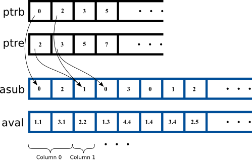
Fig. 15.1 The matrix \(A\) (15.1) represented in column ordered packed sparse matrix format.

Column ordered sparse format with nonzeros

Note that nzc[j] := ptre[j]-ptrb[j] is exactly the number of nonzero elements in the \(j\)-th column of \(A\). In some functions a sparse matrix will be represented using the equivalent dataset asub, aval, ptrb, nzc. The matrix \(A\) (15.1) would now be represented as:

\[\begin{split}\begin{array}{lcl} \mathtt{ptrb} & = & [ 0, 2, 3, 5, 7 ],\\ \mathtt{nzc} & = & [ 2, 1, 2, 2, 1 ], \\ \mathtt{asub} & = & [ 0, 2, 1, 0, 3, 0, 2, 1 ], \\ \mathtt{aval} & = & [ 1.1, 3.1, 2.2, 1.3, 4.4, 1.4, 3.4, 2.5 ]. \end{array}\end{split}\]

Row ordered sparse matrix

The matrix \(A\) (15.1) can also be represented in the row ordered sparse matrix format as:

\[\begin{split}\begin{array} {lcl} \mathtt{ptrb} & = & [ 0, 3, 5, 7 ], \\ \mathtt{ptre} & = & [ 3, 5, 7, 8 ], \\ \mathtt{asub} & = & [ 0, 2, 3, 1, 4, 0, 3, 2 ], \\ \mathtt{aval} & = & [ 1.1, 1.3, 1.4, 2.2, 2.5, 3.1, 3.4, 4.4 ]. \end{array}\end{split}\]