11.3 2D Total Variation
This case study is based mainly on the paper by Goldfarb and Yin [GY05].
Mathematical Formulation
We are given a \(n\times m\) grid and for each cell \((i,j)\) an observed value \(f_{ij}\) that can expressed as
where \(u_{ij}\in[0,1]\) is the actual signal value and \(v_{ij}\) is the noise. The aim is to reconstruct \(u\) subtracting the noise from the observations.
We assume the \(2\)-norm of the overall noise to be bounded: the corresponding constraint is
which translates into a simple conic quadratic constraint as
We aim to minimize the change in signal value when moving between adjacent cells. To this end we define the adjacent differences vector as
for each cell \(1\leq i,j\leq n\) (we assume that the respective coordinates \(\partial^x_{ij}\) and \(\partial^y_{ij}\) are zero on the right and bottom boundary of the grid).
For each cell we want to minimize the norm of \(\partial^+_{ij}\), and therefore we introduce auxiliary variables \(t_{ij}\) such that
and minimize the sum of all \(t_{ij}\).
The complete model takes the form:
Implementation
The Fusion implementation of model (11.16) uses variable and expression slices.
First of all we start by creating the optimization model and variables t and u. Since we intend to solve the problem many times with various input data we define \(\sigma\) and \(f\) as parameters:
    Model M = new Model("TV");

    Variable u = M.variable("u", new int[] {n + 1, m + 1}, Domain.inRange(0., 1.0));
    Variable t = M.variable("t", new int[] {n, m}, Domain.unbounded());

    // In this example we define sigma and the input image f as parameters
    // to demonstrate how to solve the same model with many data variants.
    // Of course they could simply be passed as ordinary arrays if that is not needed.
    Parameter sigma = M.parameter("sigma");
    Parameter f = M.parameter("f", n, m);
Note the dimensions of u is larger than those of the grid to accommodate the boundary conditions later. The actual cells of the grid are defined as a slice of u:
Variable ucore = u.slice(new int[] {0, 0}, new int[] {n, m});
The next step is to define the partial variation along each axis, as in (11.15):
    Expression deltax = Expr.sub( u.slice( new int[] {1, 0}, new int[] {n + 1, m} ), ucore );
    Expression deltay = Expr.sub( u.slice( new int[] {0, 1}, new int[] {n, m + 1} ), ucore );
Slices are created on the fly as they will not be reused. Now we can set the conic constraints on the norm of the total variations. To this extent we stack the variables t, deltax and deltay together and demand that each row of the new matrix is in a quadratic cone.
M.constraint( Expr.stack(2, t, deltax, deltay), Domain.inQCone().axis(2) );
We now need to bound the norm of the noise. This can be achieved with a conic constraint using f as a one-dimensional array:
    M.constraint( Expr.vstack(sigma, Expr.flatten( Expr.sub(f,  ucore) ) ),
                  Domain.inQCone() );
The objective function is the sum of all \(t_{ij}\):
M.objective( ObjectiveSense.Minimize, Expr.sum(t) );
Example
Consider the linear signal \(u_{ij}=\frac{i+j}{n+m}\) and its modification with random Gaussian noise, as in Fig. 11.4. Various reconstructions of \(u\), obtained with different values of \(\sigma\), are shown in Fig. 11.5 (where \(\bar{\sigma}=\sigma/nm\) is the relative noise bound per cell).
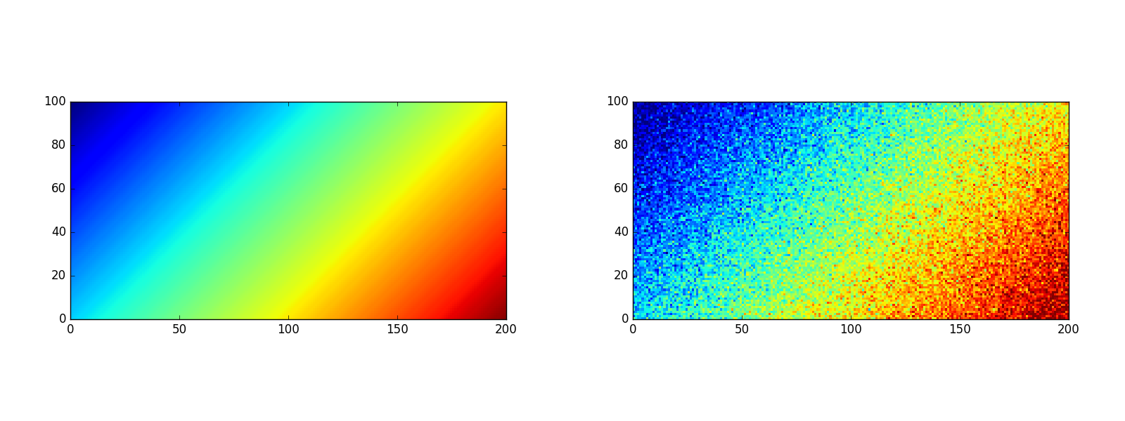
Fig. 11.4 A linear signal and its modification with random Gaussian noise.
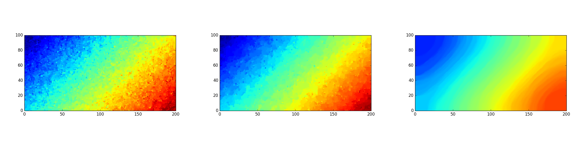
Fig. 11.5 Three reconstructions of the linear signal obtained for \(\bar{\sigma}\in\{0.0004,0.0005,0.0006\}\), respectively.
Source code
public class total_variation {

  public static Model total_var(int n, int m) {
    Model M = new Model("TV");

    Variable u = M.variable("u", new int[] {n + 1, m + 1}, Domain.inRange(0., 1.0));
    Variable t = M.variable("t", new int[] {n, m}, Domain.unbounded());

    // In this example we define sigma and the input image f as parameters
    // to demonstrate how to solve the same model with many data variants.
    // Of course they could simply be passed as ordinary arrays if that is not needed.
    Parameter sigma = M.parameter("sigma");
    Parameter f = M.parameter("f", n, m);

    Variable ucore = u.slice(new int[] {0, 0}, new int[] {n, m});

    Expression deltax = Expr.sub( u.slice( new int[] {1, 0}, new int[] {n + 1, m} ), ucore );
    Expression deltay = Expr.sub( u.slice( new int[] {0, 1}, new int[] {n, m + 1} ), ucore );

    M.constraint( Expr.stack(2, t, deltax, deltay), Domain.inQCone().axis(2) );

    M.constraint( Expr.vstack(sigma, Expr.flatten( Expr.sub(f,  ucore) ) ),
                  Domain.inQCone() );

    M.objective( ObjectiveSense.Minimize, Expr.sum(t) );

    return M;
  }

  public static void main(String[] args)
  throws SolutionError {
    Random randGen = new Random(0);

    int n = 100;
    int m = 200;
    double[] sigmas = { 0.0004, 0.0005, 0.0006 };

    // Create a parametrized model with given shape
    Model M = total_var(n, m);
    Parameter sigma = M.getParameter("sigma");
    Parameter f     = M.getParameter("f");
    Variable  ucore = M.getVariable("u").slice(new int[] {0,0}, new int[] {n,m});

    // Example: Linear signal with Gaussian noise
    double[][] signal = new double[n][m];
    double[][] noise  = new double[n][m];
    double[][] fVal   = new double[n][m];
    double[][] sol    = new double[n][m];

    for(int i=0; i<n; i++) for(int j=0; j<m; j++) {
      signal[i][j] = 1.0*(i+j)/(n+m);
      noise[i][j] = randGen.nextGaussian() * 0.08;
      fVal[i][j] = Math.max( Math.min(1.0, signal[i][j] + noise[i][j]), .0 );
    }

    // Set value for f
    f.setValue(fVal);

    for(int iter=0; iter<3; iter++) {
      // Set new value for sigma and solve
      sigma.setValue(sigmas[iter]*n*m);

      M.solve();

      // Retrieve solution from ucore
      double[] ucoreLev = ucore.level();
      for(int i=0; i<n; i++) for(int j=0; j<m; j++)
        sol[i][j] = ucoreLev[i*n+m];

      // Use the solution
      // ...

      System.out.printf("rel_sigma = %f  total_var = %.3f\n", sigmas[iter], M.primalObjValue());
    }

    M.dispose();
  }
}