10.2 Least Squares and Other Norm Minimization Problems
A frequently occurring problem in statistics and in many other areas of science is a norm minimization problem
where \(x\in\real^n\) and of course we can allow other types of constraints. The objective can involve various norms: infinity norm, 1-norm, 2-norm, \(p\)-norms and so on. For instance the most popular case of the 2-norm corresponds to the least squares linear regression, since it is equivalent to minimization of \(\|Fx-g\|_2^2\).
10.2.1 Least squares, 2-norm
In the case of the 2-norm we specify the problem directly in conic quadratic form
The first constraint of the problem can be represented as an affine conic constraint. This leads to the following model.
# Least squares regression
# minimize \|Fx-g\|_2
norm_lse <- function(F,g,A,b)
{
    n <- dim(F)[2]
    k <- length(g)
    m <- dim(A)[1]

    # Linear constraints in [x; t]
    prob <- list(sense="min")
    prob$A <- cbind(A, rep(0, m))
    prob$bx <- rbind(rep(-Inf, n+1), rep(Inf, n+1))
    prob$bc <- rbind(b, b)
    prob$c <- c(rep(0, n), 1)

    # Affine conic constraint
    prob$F <- rbind( c(rep(0,n), 1),
                     cbind(F, rep(0, k)) )
    prob$g <- c(0, -g)
    prob$cones <- matrix(list("QUAD", k+1, NULL))
    rownames(prob$cones) <- c("type","dim","conepar")

    # Solve
    r <- mosek(prob, list(verbose=1))
    stopifnot(identical(r$response$code, 0))
    r$sol$itr$xx[1:n]
}
10.2.2 Ridge regularisation
Regularisation is classically applied to reduce the impact of outliers and to control overfitting. In the conic version of ridge (Tychonov) regression we consider the problem
which can be written explicitly as
The implementation is a small extension of that from the previous section.
# Least squares regression with regularization
# minimize \|Fx-g\|_2 + gamma*\|x\|_2
norm_lse_reg <- function(F,g,A,b,gamma)
{
    n <- dim(F)[2]
    k <- length(g)
    m <- dim(A)[1]

    # Linear constraints in [x; t1; t2]
    prob <- list(sense="min")
    prob$A <- cbind(A, rep(0, m), rep(0, m))
    prob$bx <- rbind(rep(-Inf, n+2), rep(Inf, n+2))
    prob$bc <- rbind(b, b)
    prob$c <- c(rep(0, n), 1, gamma)

    # Affine conic constraint
    prob$F <- rbind(     c(rep(0,n), 1,         0),
                     cbind(F,        rep(0, k), rep(0, k)),
                         c(rep(0,n), 0,         1),
                     cbind(diag(n),  rep(0, n), rep(0, n)))
    prob$g <- c(0, -g, rep(0, n+1))
    prob$cones <- cbind(matrix(list("QUAD", k+1, NULL)),
                        matrix(list("QUAD", n+1, NULL)))
    rownames(prob$cones) <- c("type","dim","conepar")

    # Solve
    r <- mosek(prob, list(verbose=1))
    stopifnot(identical(r$response$code, 0))
    r$sol$itr$xx[1:n]
}
Note that classically least squares problems are formulated as quadratic problems and then the objective function would be written as
This version can easily be obtained by replacing the quadratic cone with an appropriate rotated quadratic cone in (10.16). Then they core of the implementation would change as follows:
    # Affine conic constraint
    prob$F <- rbind(     c(rep(0,n), 1,         0),
                         c(rep(0, n+2)),
                     cbind(F,        rep(0, k), rep(0, k)),
                         c(rep(0,n), 0,         1),
                         c(rep(0, n+2)),
                     cbind(diag(n),  rep(0, n), rep(0, n)))
    prob$g <- c(0, 0.5, -g, 0, 0.5, rep(0, n))
    prob$cones <- cbind(matrix(list("RQUAD", k+2, NULL)),
                        matrix(list("RQUAD", n+2, NULL)))
    rownames(prob$cones) <- c("type","dim","conepar")
Fig. 10.2 shows the solution to a polynomial fitting problem for a few variants of least squares regression with and without ridge regularization.
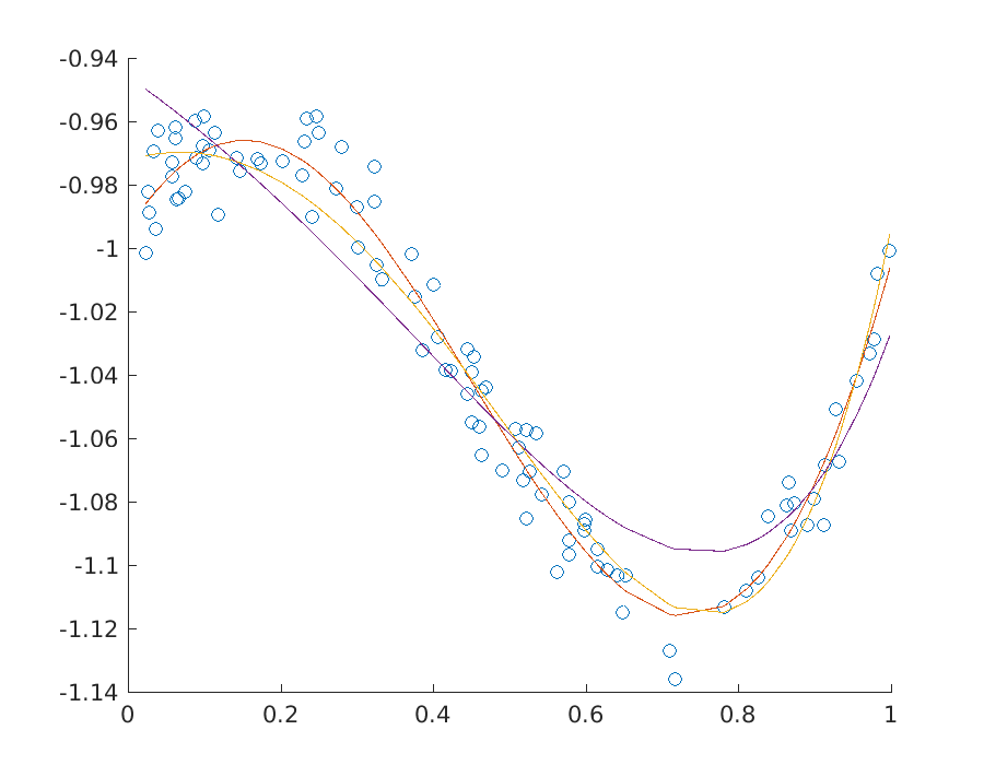
Fig. 10.2 Three fits to a dataset at various levels of regularization.
10.2.3 Lasso regularization
In lasso or least absolute shrinkage and selection operator the regularization term is the 1-norm of the solution
This variant typically tends to give preference to sparser solutions, i.e. solutions where only a few elements of \(x\) are nonzero, and therefore it is used as an efficient approximation to the cardinality constrained problem with an upper bound on the 0-norm of \(x\). To see how it works we first implement (10.17) adding the constraint \(t\geq \|x\|_1\) as a series of linear constraints
so that eventually the problem becomes
# Least squares regression with lasso regularization
# minimize \|Fx-g\|_2 + gamma*\|x\|_1
norm_lse_lasso <- function(F,g,A,b,gamma)
{
    n <- dim(F)[2]
    k <- length(g)
    m <- dim(A)[1]

    # Linear constraints in [x; u; t1; t2]
    prob <- list(sense="min")
    prob$A <- rbind(cbind(A,    matrix(0, m, n+2)),
                    cbind(diag(n), diag(n), matrix(0, n, 2)),
                    cbind(-diag(n), diag(n), matrix(0, n, 2)),
                    c(rep(0, n), rep(-1, n), 0, 1))
    prob$bx <- rbind(rep(-Inf, 2*n+2), rep(Inf, 2*n+2))
    prob$bc <- rbind(c(b, rep(0, 2*n+1)), c(b, rep(Inf, 2*n+1)))
    prob$c <- c(rep(0, 2*n), 1, gamma)

    # Affine conic constraint
    prob$F <- rbind(c(rep(0, 2*n), 1, 0),
                    cbind(F, matrix(0, k, n+2)))
    prob$g <- c(0, -g)
    prob$cones <- matrix(list("QUAD", k+1, NULL))
    rownames(prob$cones) <- c("type","dim","conepar")

    # Solve
    r <- mosek(prob, list(verbose=1))
    stopifnot(identical(r$response$code, 0))
    r$sol$itr$xx[1:n]
}
The sparsity pattern of the solution of a large random regression problem can look for example as follows:
Lasso regularization
Gamma 0.0100  density 99%   |Fx-g|_2: 54.3722
Gamma 0.1000  density 87%   |Fx-g|_2: 54.3939
Gamma 0.3000  density 67%   |Fx-g|_2: 54.5319
Gamma 0.6000  density 40%   |Fx-g|_2: 54.8379
Gamma 0.9000  density 26%   |Fx-g|_2: 55.0720
Gamma 1.3000  density 12%   |Fx-g|_2: 55.1903
10.2.4 p-norm minimization
Now we consider the minimization of the \(p\)-norm defined for \(p>1\) as
We have the optimization problem:
Increasing the value of \(p\) forces stronger penalization of outliers as ultimately, when \(p\to\infty\), the \(p\)-norm \(\|y\|_p\) converges to the infinity norm \(\|y\|_\infty\) of \(y\). According to the Modeling Cookbook the \(p\)-norm bound \(t\geq \|Fx-g\|_p\) can be added to the model using a sequence of three-dimensional power cones and we obtain an equivalent problem
The power cones can be added one by one to the structure representing affine conic constraints. Each power cone will require one \(r_i\), one copy of \(t\) and one row from \(F\) and \(g\). An alternative solution is to create the vector
and then reshuffle its elements into
using an appropriate permutation matrix. This approach is demonstrated in the code below.
# P-norm minimization
# minimize \|Fx-g\|_p
norm_p_norm <- function(F,g,A,b,p)
{
    n <- dim(F)[2]
    k <- length(g)
    m <- dim(A)[1]

    # Linear constraints in [x; r; t]
    prob <- list(sense="min")
    prob$A <- rbind(cbind(A,    matrix(0, m, k+1)),
                    c(rep(0, n), rep(1, k), -1))
    prob$bx <- rbind(rep(-Inf, n+k+1), rep(Inf, n+k+1))
    prob$bc <- rbind(c(b, 0), c(b, 0))
    prob$c <- c(rep(0, n+k), 1)

    # Permutation matrix which picks triples (r_i, t, F_ix-g_i)
    M <- cbind(sparseMatrix(seq(1,3*k,3), seq(1,k), x=rep(1,k), dims=c(3*k,k)),
               sparseMatrix(seq(2,3*k,3), seq(1,k), x=rep(1,k), dims=c(3*k,k)),
               sparseMatrix(seq(3,3*k,3), seq(1,k), x=rep(1,k), dims=c(3*k,k)))

    # Affine conic constraint
    prob$F <- M %*% rbind(cbind(matrix(0, k, n), diag(k), rep(0, k)),
                          cbind(matrix(0, k, n+k), rep(1, k)),
                          cbind(F, matrix(0, k, k+1)))
    prob$g <- as.numeric(M %*% c(rep(0, 2*k), -g))
    prob$cones <- matrix(list("PPOW", 3, c(1, p-1)), nrow=3, ncol=k)
    rownames(prob$cones) <- c("type","dim","conepar")

    # Solve
    r <- mosek(prob, list(verbose=1))
    stopifnot(identical(r$sol$itr$prosta, "PRIMAL_AND_DUAL_FEASIBLE"))
    r$sol$itr$xx[1:n]
}
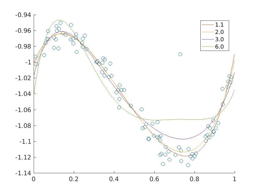
Fig. 10.3 \(p\)-norm minimizing fits of a polynomial of degree at most 5 to the data for various values of \(p\).