14.3 Sensitivity Analysis

Given an optimization problem it is often useful to obtain information about how the optimal objective value changes when the problem parameters are perturbed. E.g, assume that a bound represents the capacity of a machine. Now, it may be possible to expand the capacity for a certain cost and hence it is worthwhile knowing what the value of additional capacity is. This is precisely the type of questions the sensitivity analysis deals with.

Analyzing how the optimal objective value changes when the problem data is changed is called sensitivity analysis.

References

The book [Chvatal83] discusses the classical sensitivity analysis in Chapter 10 whereas the book [RTV97] presents a modern introduction to sensitivity analysis. Finally, it is recommended to read the short paper [Wal00] to avoid some of the pitfalls associated with sensitivity analysis.

Warning

Currently, sensitivity analysis is only available for continuous linear optimization problems. Moreover, MOSEK can only deal with perturbations of bounds and objective function coefficients.

14.3.1 Sensitivity Analysis for Linear Problems

14.3.1.1 The Optimal Objective Value Function

Assume that we are given the problem

(14.3)\[\begin{split}\begin{array}{rclccccl} z(l^c,u^c,l^x,u^x,c) & = & \mbox{minimize} & & & c^Tx & & \\ & & \mbox{subject to} & l^c & \leq & Ax & \leq & u^c, \\ & & & l^x & \leq & x & \leq & u^x, \end{array}\end{split}\]

and we want to know how the optimal objective value changes as \(l^c_i\) is perturbed. To answer this question we define the perturbed problem for \(l^c_i\) as follows

\[\begin{split}\begin{array}{rclcccl} f_{l^c_i}(\beta ) & = & \mbox{minimize} & & & c^Tx & \\ & & \mbox{subject to} & l^c + \beta e_i & \leq & Ax & \leq u^c, \\ & & & l^x & \leq & x \leq & u^x, \end{array}\end{split}\]

where \(e_i\) is the \(i\)-th column of the identity matrix. The function

(14.4)\[f_{l^c_i}(\beta)\]

shows the optimal objective value as a function of \(\beta\). Please note that a change in \(\beta\) corresponds to a perturbation in \(l_i^c\) and hence (14.4) shows the optimal objective value as a function of varying \(l^c_i\) with the other bounds fixed.

It is possible to prove that the function (14.4) is a piecewise linear and convex function, i.e. its graph may look like in Fig. 14.1 and Fig. 14.2.

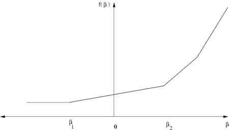
Fig. 14.1 \(\beta =0\) is in the interior of linearity interval.

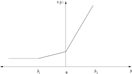
Fig. 14.2 \(\beta =0\) is a breakpoint.

Clearly, if the function \(f_{l^c_i}(\beta )\) does not change much when \(\beta\) is changed, then we can conclude that the optimal objective value is insensitive to changes in \(l_i^c\). Therefore, we are interested in the rate of change in \(f_{l^c_i}(\beta)\) for small changes in \(\beta\) — specifically the gradient

\[f^\prime_{l^c_i}(0),\]

which is called the shadow price related to \(l^c_i\). The shadow price specifies how the objective value changes for small changes of \(\beta\) around zero. Moreover, we are interested in the linearity interval

\[\beta \in [\beta_1,\beta_2]\]

for which

\[f^\prime_{l^c_i}(\beta ) = f^\prime_{l^c_i}(0).\]

Since \(f_{l^c_i}\) is not a smooth function \(f^\prime_{l^c_i}\) may not be defined at \(0\), as illustrated in Fig. 14.2. In this case we can define a left and a right shadow price and a left and a right linearity interval.

The function \(f_{l^c_i}\) considered only changes in \(l^c_i\). We can define similar functions for the remaining parameters of the \(z\) defined in (14.3) as well:

\[\begin{split}\begin{array}{rcll} f_{l^c_i}(\beta ) & = & z(l^c+\beta e_i,u^c,l^x,u^x,c), & i=1,\ldots,m, \\ f_{u^c_i}(\beta ) & = & z(l^c,u^c+\beta e_i,l^x,u^x,c), & i=1,\ldots,m, \\ f_{l^x_{j}}(\beta ) & = & z(l^c,u^c,l^x+\beta e_{j},u^x,c), & j=1,\ldots,n, \\ f_{u^x_{j}}(\beta ) & = & z(l^c,u^c,l^x,u^x+\beta e_{j},c), & j=1,\ldots,n, \\ f_{c_{j}}(\beta ) & = & z(l^c,u^c,l^x,u^x,c+\beta e_{j}), & j=1,\ldots,n. \end{array}\end{split}\]

Given these definitions it should be clear how linearity intervals and shadow prices are defined for the parameters \(u^c_i\) etc.

14.3.1.1.1 Equality Constraints

In MOSEK a constraint can be specified as either an equality constraint or a ranged constraint. If some constraint \(e_i^c\) is an equality constraint, we define the optimal value function for this constraint as

\[f_{e_i^c}(\beta ) = z(l^c+\beta e_i,u^c+\beta e_i,l^x,u^x,c)\]

Thus for an equality constraint the upper and the lower bounds (which are equal) are perturbed simultaneously. Therefore, MOSEK will handle sensitivity analysis differently for a ranged constraint with \(l^c_i = u^c_i\) and for an equality constraint.

14.3.1.2 The Basis Type Sensitivity Analysis

The classical sensitivity analysis discussed in most textbooks about linear optimization, e.g. [Chvatal83], is based on an optimal basis. This method may produce misleading results [RTV97] but is computationally cheap. This is the type of sensitivity analysis implemented in MOSEK.

We will now briefly discuss the basis type sensitivity analysis. Given an optimal basic solution which provides a partition of variables into basic and non-basic variables, the basis type sensitivity analysis computes the linearity interval \([\beta_1,\beta_2]\) so that the basis remains optimal for the perturbed problem. A shadow price associated with the linearity interval is also computed. However, it is well-known that an optimal basic solution may not be unique and therefore the result depends on the optimal basic solution employed in the sensitivity analysis. If the optimal objective value function has a breakpoint for \(\beta = 0\) then the basis type sensitivity method will only provide a subset of either the left or the right linearity interval.

In summary, the basis type sensitivity analysis is computationally cheap but does not provide complete information. Hence, the results of the basis type sensitivity analysis should be used with care.

14.3.1.3 Example: Sensitivity Analysis

As an example we will use the following transportation problem. Consider the problem of minimizing the transportation cost between a number of production plants and stores. Each plant supplies a number of goods and each store has a given demand that must be met. Supply, demand and cost of transportation per unit are shown in Fig. 14.3.

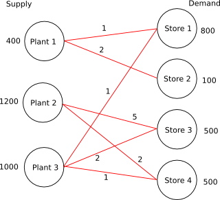
Fig. 14.3 Supply, demand and cost of transportation.

If we denote the number of transported goods from location \(i\) to location \(j\) by \(x_{ij}\), problem can be formulated as the linear optimization problem of minimizing

\[\begin{array}{ccccccccccccc} 1x_{11} & + & 2x_{12} & + & 5x_{23} & + & 2x_{24} & + & 1x_{31} & + & 2x_{33} & + & 1 x_{34} \end{array}\]

subject to

(14.5)\[\begin{split}\begin{array}{ccccccccccccccl} x_{11} & + & x_{12} & & & & & & & & & & & \leq & 400, \\ & & & & x_{23} & + & x_{24} & & & & & & & \leq & 1200, \\ & & & & & & & & x_{31} & + & x_{33} & + & x_{34} & \leq & 1000, \\ x_{11} & & & & & & & + & x_{31} & & & & & = & 800, \\ & & x_{12} & & & & & & & & & & & = & 100, \\ & & & & x_{23} & + & & & & & x_{33} & & & = & 500, \\ & & & & & & x_{24} & + & & & & & x_{34} & = & 500, \\ x_{11}, & & x_{12}, & & x_{23}, & & x_{24}, & & x_{31}, & & x_{33}, & & x_{34} & \geq & 0. \end{array}\end{split}\]

The sensitivity parameters are shown in Table 14.1 and Table 14.2.

Table 14.1 Ranges and shadow prices related to bounds on constraints and variables.

Con.	\(\beta_1\)	\(\beta_2\)	\(\sigma_1\)	\(\sigma_2\)
\(1\)	\(-300.00\)	\(0.00\)	\(3.00\)	\(3.00\)
\(2\)	\(-700.00\)	\(+\infty\)	\(0.00\)	\(0.00\)
\(3\)	\(-500.00\)	\(0.00\)	\(3.00\)	\(3.00\)
\(4\)	\(-0.00\)	\(500.00\)	\(4.00\)	\(4.00\)
\(5\)	\(-0.00\)	\(300.00\)	\(5.00\)	\(5.00\)
\(6\)	\(-0.00\)	\(700.00\)	\(5.00\)	\(5.00\)
\(7\)	\(-500.00\)	\(700.00\)	\(2.00\)	\(2.00\)
Var.	\(\beta_1\)	\(\beta_2\)	\(\sigma_1\)	\(\sigma_2\)
\(x_{11}\)	\(-\infty\)	\(300.00\)	\(0.00\)	\(0.00\)
\(x_{12}\)	\(-\infty\)	\(100.00\)	\(0.00\)	\(0.00\)
\(x_{23}\)	\(-\infty\)	\(0.00\)	\(0.00\)	\(0.00\)
\(x_{24}\)	\(-\infty\)	\(500.00\)	\(0.00\)	\(0.00\)
\(x_{31}\)	\(-\infty\)	\(500.00\)	\(0.00\)	\(0.00\)
\(x_{33}\)	\(-\infty\)	\(500.00\)	\(0.00\)	\(0.00\)
\(x_{34}\)	\(-0.000000\)	\(500.00\)	\(2.00\)	\(2.00\)

Table 14.2 Ranges and shadow prices related to the objective coefficients.

Var.	\(\beta_1\)	\(\beta_2\)	\(\sigma_1\)	\(\sigma_2\)
\(c_1\)	\(-\infty\)	\(3.00\)	\(300.00\)	\(300.00\)
\(c_2\)	\(-\infty\)	\(\infty\)	\(100.00\)	\(100.00\)
\(c_3\)	\(-2.00\)	\(\infty\)	\(0.00\)	\(0.00\)
\(c_4\)	\(-\infty\)	\(2.00\)	\(500.00\)	\(500.00\)
\(c_5\)	\(-3.00\)	\(\infty\)	\(500.00\)	\(500.00\)
\(c_6\)	\(-\infty\)	\(2.00\)	\(500.00\)	\(500.00\)
\(c_7\)	\(-2.00\)	\(\infty\)	\(0.00\)	\(0.00\)

Examining the results from the sensitivity analysis we see that for constraint number \(1\) we have \(\sigma_1 = 3\) and \(\beta_1 = -300,\ \beta_2=0\).

If the upper bound on constraint \(1\) is decreased by

\[\beta \in [0,300]\]

then the optimal objective value will increase by the value

\[\sigma_1 \beta = 3 \beta .\]

14.3.2 Sensitivity Analysis with MOSEK

MOSEK provides the functions Task.primalsensitivity and Task.dualsensitivity for performing sensitivity analysis. The code in Listing 14.2 gives an example of its use.

Listing 14.2 Example of sensitivity analysis with the MOSEK Optimizer API for Java. Click here to download.

package com.mosek.example;
import mosek.*;

public class sensitivity {
  public static void main (String[] args) {
    // Since the value infinity is never used, we define
    // 'infinity' symbolic purposes only
    double
    infinity = 0;

    try (Task task = new Task()) {
      mosek.boundkey[] bkc = {
        mosek.boundkey.up, mosek.boundkey.up,
        mosek.boundkey.up, mosek.boundkey.fx,
        mosek.boundkey.fx, mosek.boundkey.fx,
        mosek.boundkey.fx
      };
      mosek.boundkey[] bkx = {
        mosek.boundkey.lo, mosek.boundkey.lo,
        mosek.boundkey.lo, mosek.boundkey.lo,
        mosek.boundkey.lo, mosek.boundkey.lo,
        mosek.boundkey.lo
      };
      int[] ptrb = {0, 2, 4, 6, 8, 10, 12};
      int[] ptre = {2, 4, 6, 8, 10, 12, 14};
      int[] sub = {0, 3, 0, 4, 1, 5, 1, 6, 2, 3, 2, 5, 2, 6};
      double[] blc = { -infinity, -infinity,
                       -infinity, 800, 100, 500, 500
                     };
      double[] buc = {400, 1200, 1000, 800, 100, 500, 500};
      double[] c   = {1.0, 2.0, 5.0, 2.0, 1.0, 2.0, 1.0};
      double[] blx = {0.0, 0.0, 0.0, 0.0, 0.0, 0.0, 0.0};
      double[] bux = {infinity, infinity,
                      infinity, infinity,
                      infinity, infinity,
                      infinity
                     };
      double[] val = {1.0, 1.0, 1.0, 1.0, 1.0, 1.0, 1.0,
                      1.0, 1.0, 1.0, 1.0, 1.0, 1.0, 1.0
                     };

      int numcon = 7;  /* Number of constraints.             */
      int numvar = 7;  /* Number of variables.               */
      int NUMANZ = 14; /* Number of non-zeros in A.           */

      // Directs the log task stream to the user specified
      // method task_msg_obj.print
      task.set_Stream(
        mosek.streamtype.log,
        new mosek.Stream()
      { public void stream(String msg) { System.out.print(msg); }});

      task.inputdata(numcon, numvar,
                     c,
                     0.0,
                     ptrb,
                     ptre,
                     sub,
                     val,
                     bkc,
                     blc,
                     buc,
                     bkx,
                     blx,
                     bux);

      /* A maximization problem */
      task.putobjsense(mosek.objsense.minimize);

      task.optimize();

      /* Analyze upper bound on c1 and the equality constraint on c4 */
      int subi[]  = {0, 3};
      mosek.mark marki[] = {mosek.mark.up, mosek.mark.up};

      /* Analyze lower bound on the variables x12 and x31 */
      int subj[]  = {1, 4};
      mosek.mark markj[] = {mosek.mark.lo, mosek.mark.lo};

      double[] leftpricei  = new  double[2];
      double[] rightpricei  = new  double[2];
      double[] leftrangei  = new  double[2];
      double[] rightrangei = new  double[2];
      double[] leftpricej  = new  double[2];
      double[] rightpricej = new  double[2];
      double[] leftrangej  = new  double[2];
      double[] rightrangej = new  double[2];


      task.primalsensitivity( subi,
                              marki,
                              subj,
                              markj,
                              leftpricei,
                              rightpricei,
                              leftrangei,
                              rightrangei,
                              leftpricej,
                              rightpricej,
                              leftrangej,
                              rightrangej);

      System.out.println("Results from sensitivity analysis on bounds:\n");

      System.out.println("For constraints:\n");
      for (int i = 0; i < 2; ++i)
        System.out.print("leftprice = " + leftpricei[i] +
                         " rightprice = " + rightpricei[i] +
                         " leftrange = " + leftrangei[i] +
                         " rightrange = " + rightrangei[i] + "\n");

      System.out.print("For variables:\n");
      for (int i = 0; i < 2; ++i)
        System.out.print("leftprice = " + leftpricej[i] +
                         " rightprice = " + rightpricej[i] +
                         " leftrange = " + leftrangej[i] +
                         " rightrange = " + rightrangej[i] + "\n");


      double[] leftprice  = new  double[2];
      double[] rightprice = new  double[2];
      double[] leftrange  = new  double[2];
      double[] rightrange = new  double[2];
      int subc[]  = {2, 5};

      task.dualsensitivity(  subc,
                             leftprice,
                             rightprice,
                             leftrange,
                             rightrange
                          );

      System.out.println(
        "Results from sensitivity analysis on objective coefficients:"
      );

      for (int i = 0; i < 2; ++i)
        System.out.print("leftprice = " + leftprice[i] +
                         " rightprice = " + rightprice[i] +
                         " leftrange = " + leftrange[i] +
                         " rightrange = " +  rightrange[i] + "\n");


    } catch (mosek.Exception e)
      /* Catch both mosek.Error and mosek.Warning */
    {
      System.out.println ("An error or warning was encountered");
      System.out.println (e.getMessage ());
      throw e;
    }
  }
}