9.3 Sensitivity Analysis

Given an optimization problem it is often useful to obtain information about how the optimal objective value changes when the problem parameters are perturbed. E.g, assume that a bound represents the capacity of a machine. Now, it may be possible to expand the capacity for a certain cost and hence it is worthwhile knowing what the value of additional capacity is. This is precisely the type of questions the sensitivity analysis deals with.

Analyzing how the optimal objective value changes when the problem data is changed is called sensitivity analysis.

References

The book [Chvatal83] discusses the classical sensitivity analysis in Chapter 10 whereas the book [RTV97] presents a modern introduction to sensitivity analysis. Finally, it is recommended to read the short paper [Wal00] to avoid some of the pitfalls associated with sensitivity analysis.

Warning

Currently, sensitivity analysis is only available for continuous linear optimization problems. Moreover, MOSEK can only deal with perturbations of bounds and objective function coefficients.

9.3.1 Sensitivity Analysis for Linear Problems

9.3.1.1 The Optimal Objective Value Function

Assume that we are given the problem

(9.3)$$\begin{array}{r}\begin{array}{rclccccl}z(l^c,u^c,l^x,u^x,c)& =& \text{minimize}& & & c^{T}x& & \\ & & \text{subject to}& l^c& \le & Ax& \le & u^c,\\ & & & l^x& \le & x& \le & u^x,\end{array}\end{array}$$

and we want to know how the optimal objective value changes as $l_i^c$ is perturbed. To answer this question we define the perturbed problem for $l_i^c$ as follows

$$\begin{array}{r}\begin{array}{rclcccl}{f}_{l_i^c}(\beta )& =& \text{minimize}& & & c^{T}x& \\ & & \text{subject to}& l^c+\beta e_i& \le & Ax& \le u^c,\\ & & & l^x& \le & x\le & u^x,\end{array}\end{array}$$

where $e_i$ is the $i$-th column of the identity matrix. The function

(9.4)$$f_{l_i^c}(\beta )$$

shows the optimal objective value as a function of $\beta$. Please note that a change in $\beta$ corresponds to a perturbation in $l_i^c$ and hence (9.4) shows the optimal objective value as a function of varying $l_i^c$ with the other bounds fixed.

It is possible to prove that the function (9.4) is a piecewise linear and convex function, i.e. its graph may look like in Fig. 9.1 and Fig. 9.2.

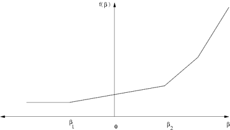
Fig. 9.1 $\beta =0$ is in the interior of linearity interval.

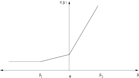
Fig. 9.2 $\beta =0$ is a breakpoint.

Clearly, if the function $f_{l_i^c}(\beta )$ does not change much when $\beta$ is changed, then we can conclude that the optimal objective value is insensitive to changes in $l_i^c$. Therefore, we are interested in the rate of change in $f_{l_i^c}(\beta )$ for small changes in $\beta$ — specifically the gradient

$$f_{l_i^c}^{\prime }(0),$$

which is called the shadow price related to $l_i^c$. The shadow price specifies how the objective value changes for small changes of $\beta$ around zero. Moreover, we are interested in the linearity interval

$$\beta \in [{\beta }_1,{\beta }_2]$$

for which

$$f_{l_i^c}^{\prime }(\beta )=f_{l_i^c}^{\prime }(0).$$

Since $f_{l_i^c}$ is not a smooth function $f_{l_i^c}^{\prime }$ may not be defined at $0$, as illustrated in Fig. 9.2. In this case we can define a left and a right shadow price and a left and a right linearity interval.

The function $f_{l_i^c}$ considered only changes in $l_i^c$. We can define similar functions for the remaining parameters of the $z$ defined in (9.3) as well:

$$\begin{array}{r}\begin{array}{rcll}{f}_{l_i^c}(\beta )& =& z(l^c+\beta e_i,u^c,l^x,u^x,c),& i=1,\dots ,m,\\ f_{u_i^c}(\beta )& =& z(l^c,u^c+\beta e_i,l^x,u^x,c),& i=1,\dots ,m,\\ f_{l_j^x}(\beta )& =& z(l^c,u^c,l^x+\beta e_j,u^x,c),& j=1,\dots ,n,\\ f_{u_j^x}(\beta )& =& z(l^c,u^c,l^x,u^x+\beta e_j,c),& j=1,\dots ,n,\\ f_{c_j}(\beta )& =& z(l^c,u^c,l^x,u^x,c+\beta e_j),& j=1,\dots ,n.\end{array}\end{array}$$

Given these definitions it should be clear how linearity intervals and shadow prices are defined for the parameters $u_i^c$ etc.

9.3.1.1.1 Equality Constraints

In MOSEK a constraint can be specified as either an equality constraint or a ranged constraint. If some constraint $e_i^c$ is an equality constraint, we define the optimal value function for this constraint as

$$f_{e_i^c}(\beta )=z(l^c+\beta e_i,u^c+\beta e_i,l^x,u^x,c)$$

Thus for an equality constraint the upper and the lower bounds (which are equal) are perturbed simultaneously. Therefore, MOSEK will handle sensitivity analysis differently for a ranged constraint with $l_i^c=u_i^c$ and for an equality constraint.

9.3.1.2 The Basis Type Sensitivity Analysis

The classical sensitivity analysis discussed in most textbooks about linear optimization, e.g. [Chvatal83], is based on an optimal basis. This method may produce misleading results [RTV97] but is computationally cheap. This is the type of sensitivity analysis implemented in MOSEK.

We will now briefly discuss the basis type sensitivity analysis. Given an optimal basic solution which provides a partition of variables into basic and non-basic variables, the basis type sensitivity analysis computes the linearity interval $[{\beta }_1,{\beta }_2]$ so that the basis remains optimal for the perturbed problem. A shadow price associated with the linearity interval is also computed. However, it is well-known that an optimal basic solution may not be unique and therefore the result depends on the optimal basic solution employed in the sensitivity analysis. If the optimal objective value function has a breakpoint for $\beta =0$ then the basis type sensitivity method will only provide a subset of either the left or the right linearity interval.

In summary, the basis type sensitivity analysis is computationally cheap but does not provide complete information. Hence, the results of the basis type sensitivity analysis should be used with care.

9.3.1.3 Example: Sensitivity Analysis

As an example we will use the following transportation problem. Consider the problem of minimizing the transportation cost between a number of production plants and stores. Each plant supplies a number of goods and each store has a given demand that must be met. Supply, demand and cost of transportation per unit are shown in Fig. 9.3.

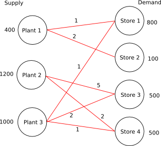
Fig. 9.3 Supply, demand and cost of transportation.

If we denote the number of transported goods from location $i$ to location $j$ by $x_{ij}$, problem can be formulated as the linear optimization problem of minimizing

$$\begin{array}{ccccccccccccc}1x_{11}& +& 2x_{12}& +& 5x_{23}& +& 2x_{24}& +& 1x_{31}& +& 2x_{33}& +& 1x_{34}\end{array}$$

subject to

(9.5)$$\begin{array}{r}\begin{array}{ccccccccccccccl}{x}_{11}& +& x_{12}& & & & & & & & & & & \le & 400,\\ & & & & x_{23}& +& x_{24}& & & & & & & \le & 1200,\\ & & & & & & & & x_{31}& +& x_{33}& +& x_{34}& \le & 1000,\\ x_{11}& & & & & & & +& x_{31}& & & & & =& 800,\\ & & x_{12}& & & & & & & & & & & =& 100,\\ & & & & x_{23}& +& & & & & x_{33}& & & =& 500,\\ & & & & & & x_{24}& +& & & & & x_{34}& =& 500,\\ x_{11},& & x_{12},& & x_{23},& & x_{24},& & x_{31},& & x_{33},& & x_{34}& \ge & 0.\end{array}\end{array}$$

The sensitivity parameters are shown in Table 9.1 and Table 9.2.

Table 9.1 Ranges and shadow prices related to bounds on constraints and variables.

Con.	${\beta }_1$	${\beta }_2$	${\sigma }_1$	${\sigma }_2$
$1$	$-300.00$	$0.00$	$3.00$	$3.00$
$2$	$-700.00$	$+\mathrm{\infty }$	$0.00$	$0.00$
$3$	$-500.00$	$0.00$	$3.00$	$3.00$
$4$	$-0.00$	$500.00$	$4.00$	$4.00$
$5$	$-0.00$	$300.00$	$5.00$	$5.00$
$6$	$-0.00$	$700.00$	$5.00$	$5.00$
$7$	$-500.00$	$700.00$	$2.00$	$2.00$
Var.	${\beta }_1$	${\beta }_2$	${\sigma }_1$	${\sigma }_2$
$x_{11}$	$-\mathrm{\infty }$	$300.00$	$0.00$	$0.00$
$x_{12}$	$-\mathrm{\infty }$	$100.00$	$0.00$	$0.00$
$x_{23}$	$-\mathrm{\infty }$	$0.00$	$0.00$	$0.00$
$x_{24}$	$-\mathrm{\infty }$	$500.00$	$0.00$	$0.00$
$x_{31}$	$-\mathrm{\infty }$	$500.00$	$0.00$	$0.00$
$x_{33}$	$-\mathrm{\infty }$	$500.00$	$0.00$	$0.00$
$x_{34}$	$-0.000000$	$500.00$	$2.00$	$2.00$

Table 9.2 Ranges and shadow prices related to the objective coefficients.

Var.	${\beta }_1$	${\beta }_2$	${\sigma }_1$	${\sigma }_2$
$c_1$	$-\mathrm{\infty }$	$3.00$	$300.00$	$300.00$
$c_2$	$-\mathrm{\infty }$	$\mathrm{\infty }$	$100.00$	$100.00$
$c_3$	$-2.00$	$\mathrm{\infty }$	$0.00$	$0.00$
$c_4$	$-\mathrm{\infty }$	$2.00$	$500.00$	$500.00$
$c_5$	$-3.00$	$\mathrm{\infty }$	$500.00$	$500.00$
$c_6$	$-\mathrm{\infty }$	$2.00$	$500.00$	$500.00$
$c_7$	$-2.00$	$\mathrm{\infty }$	$0.00$	$0.00$

Examining the results from the sensitivity analysis we see that for constraint number $1$ we have ${\sigma }_1=3$ and ${\beta }_1=-300,{\beta }_2=0$.

If the upper bound on constraint $1$ is decreased by

$$\beta \in [0,300]$$

then the optimal objective value will increase by the value

$${\sigma }_1\beta =3\beta .$$

9.3.2 Sensitivity Analysis with MOSEK

A sensitivity analysis can be performed with the MOSEK command line tool specifying the option -sen, e.g.

mosek myproblem.mps -sen sensitivity.ssp

where sensitivity.ssp is a file in the format described in the next section. The ssp file describes which parts of the problem the sensitivity analysis should be performed on, see Sec. 9.3.2.1 (Sensitivity Analysis Specification File).

By default results are written to a file named myproblem.sen. If necessary, this file name can be changed by setting the MSK_SPAR_SENSITIVITY_RES_FILE_NAME parameter.

9.3.2.1 Sensitivity Analysis Specification File

MOSEK employs an MPS-like file format to specify on which model parameters the sensitivity analysis should be performed. The format of the sensitivity specification file is shown in Listing 9.2, where capitalized names are keywords, and names in brackets are names of the constraints and variables to be included in the analysis.

Listing 9.2 Sensitivity analysis file specification.

BOUNDS CONSTRAINTS
U|L|LU [cname1]
U|L|LU [cname2]-[cname3]
BOUNDS VARIABLES
U|L|LU [vname1]
U|L|LU [vname2]-[vname3]
OBJECTIVE VARIABLES
[vname1]
[vname2]-[vname3]

The sensitivity specification file has three sections, i.e.

• BOUNDS CONSTRAINTS: Specifies on which bounds on constraints the sensitivity analysis should be performed.

• BOUNDS VARIABLES: Specifies on which bounds on variables the sensitivity analysis should be performed.

• OBJECTIVE VARIABLES: Specifies on which objective coefficients the sensitivity analysis should be performed.

A line in the body of a section must begin with a whitespace. In the BOUNDS sections one of the keys L, U, and LU must appear next. These keys specify whether the sensitivity analysis is performed on the lower bound, on the upper bound, or on both the lower and the upper bound respectively. Next, a single constraint (variable) or range of constraints (variables) is specified.

Recall from Sec. 9.3.1.1.1 (Equality Constraints) that equality constraints are handled in a special way. Sensitivity analysis of an equality constraint can be specified with either L, U, or LU, all indicating the same, namely that upper and lower bounds (which are equal) are perturbed simultaneously.

As an example consider

BOUNDS CONSTRAINTS
L  "cons1"
U  "cons2"
LU "cons3"-"cons6"

which requests that sensitivity analysis is performed on the lower bound of the constraint named cons1, on the upper bound of the constraint named cons2, and on both lower and upper bound on the constraints named cons3 to cons6.

It is allowed to use indexes instead of names, for instance

BOUNDS CONSTRAINTS
L  "cons1"
U  2
LU 3 - 6

The character * indicates that the line contains a comment and is ignored.

9.3.2.2 Example: Sensitivity Analysis from Command Line

As an example consider problem (9.5): the sensitivity file shown below (included in the distribution among the examples).

Listing 9.3 Sensitivity file for problem (9.5). Click here to download.

* Comment 1

BOUNDS CONSTRAINTS
 U "c1"         * Analyze upper bound for constraints named c1 
 U 2            * Analyze upper bound for constraints with index 2 
 U 3-5          * Analyze upper bound for constraint with index in interval [3:5] 

VARIABLES CONSTRAINTS
 L 2-4          * This section specifies which bounds on variables should be analyzed.  
 L "x11" 
OBJECTIVE CONSTRAINTS
 "x11"          * This section specifies which objective coeficients should be analysed. 
 2

The command

mosek transport.lp -sen sensitivity.ssp

produces the output file as follow

Listing 9.4 Results of sensitivity analysis

BOUNDS CONSTRAINTS
INDEX    NAME             BOUND    LEFTRANGE        RIGHTRANGE       LEFTPRICE        RIGHTPRICE
0        c1               UP       -6.574875e-18    5.000000e+02     1.000000e+00     1.000000e+00
2        c3               UP       -6.574875e-18    5.000000e+02     1.000000e+00     1.000000e+00
3        c4               FIX      -5.000000e+02    6.574875e-18     2.000000e+00     2.000000e+00
4        c5               FIX      -1.000000e+02    6.574875e-18     3.000000e+00     3.000000e+00
5        c6               FIX      -5.000000e+02    6.574875e-18     3.000000e+00     3.000000e+00

BOUNDS VARIABLES
INDEX    NAME             BOUND    LEFTRANGE        RIGHTRANGE       LEFTPRICE        RIGHTPRICE
2        x23              LO       -6.574875e-18    5.000000e+02     2.000000e+00     2.000000e+00
3        x24              LO       -inf             5.000000e+02     0.000000e+00     0.000000e+00
4        x31              LO       -inf             5.000000e+02     0.000000e+00     0.000000e+00
0        x11              LO       -inf             3.000000e+02     0.000000e+00     0.000000e+00

OBJECTIVE VARIABLES
INDEX    NAME                      LEFTRANGE        RIGHTRANGE       LEFTPRICE        RIGHTPRICE
0        x11                       -inf             1.000000e+00     3.000000e+02     3.000000e+02
2        x23                       -2.000000e+00    +inf             0.000000e+00     0.000000e+00

9.3.2.3 Controlling Log Output

Setting the parameter MSK_IPAR_LOG_SENSITIVITY to $1$ or $0$ (default) controls whether or not the results from sensitivity calculations are printed to the message stream.

The parameter MSK_IPAR_LOG_SENSITIVITY_OPT controls the amount of debug information on internal calculations from the sensitivity analysis.