11.1 Portfolio Optimization
In this section the Markowitz portfolio optimization problem and variants are implemented using Optimizer API for C.
Familiarity with Sec. 6.2 (From Linear to Conic Optimization) is recommended to follow the syntax used to create affine conic constraints (ACCs) throughout all the models appearing in this case study.
11.1.1 The Basic Model
The classical Markowitz portfolio optimization problem considers investing in \(n\) stocks or assets held over a period of time. Let \(x_j\) denote the amount invested in asset \(j\), and assume a stochastic model where the return of the assets is a random variable \(r\) with known mean
and covariance
The return of the investment is also a random variable \(y = r^Tx\) with mean (or expected return)
and variance
The standard deviation
is usually associated with risk.
The problem facing the investor is to rebalance the portfolio to achieve a good compromise between risk and expected return, e.g., maximize the expected return subject to a budget constraint and an upper bound (denoted \(\gamma\)) on the tolerable risk. This leads to the optimization problem
The variables \(x\) denote the investment i.e. \(x_j\) is the amount invested in asset \(j\) and \(x_j^0\) is the initial holding of asset \(j\). Finally, \(w\) is the initial amount of cash available.
A popular choice is \(x^0=0\) and \(w=1\) because then \(x_j\) may be interpreted as the relative amount of the total portfolio that is invested in asset \(j\).
Since \(e\) is the vector of all ones then
is the total investment. Clearly, the total amount invested must be equal to the initial wealth, which is
\[w + e^T x^0.\]
This leads to the first constraint
\[e^T x = w + e^T x^0.\]
The second constraint
\[x^T \Sigma x \leq \gamma^2\]
ensures that the variance, is bounded by the parameter \(\gamma^2\). Therefore, \(\gamma\) specifies an upper bound of the standard deviation (risk) the investor is willing to undertake. Finally, the constraint
\[x_j \geq 0\]
excludes the possibility of short-selling. This constraint can of course be excluded if short-selling is allowed.
The covariance matrix \(\Sigma\) is positive semidefinite by definition and therefore there exist a matrix \(G \in \mathbb{R}^{n\times k}\) such that
In general the choice of \(G\) is not unique and one possible choice of \(G\) is the Cholesky factorization of \(\Sigma\). However, in many cases another choice is better for efficiency reasons as discussed in Sec. 11.1.3 (Factor model and efficiency). For a given \(G\) we have that
Hence, we may write the risk constraint as
or equivalently
where \(\Q^{k+1}\) is the \((k+1)\)-dimensional quadratic cone. Note that specifically when \(G\) is derived using Cholesky factorization, \(k = n\).
Therefore, problem (11.1) can be written as
which is a conic quadratic optimization problem that can easily be formulated and solved with Optimizer API for C. Subsequently we will use the example data
and
Using Cholesky factorization, this implies
In Sec. 11.1.3 (Factor model and efficiency), we present a different way of obtaining \(G\) based on a factor model, that leads to more efficient computation.
Why a Conic Formulation?
Problem (11.1) is a convex quadratically constrained optimization problem that can be solved directly using MOSEK. Why then reformulate it as a conic quadratic optimization problem (11.3)? The main reason for choosing a conic model is that it is more robust and usually solves faster and more reliably. For instance it is not always easy to numerically validate that the matrix \(\Sigma\) in (11.1) is positive semidefinite due to the presence of rounding errors. It is also very easy to make a mistake so \(\Sigma\) becomes indefinite. These problems are completely eliminated in the conic formulation.
Moreover, observe the constraint
more numerically robust than
for very small and very large values of \(\gamma\). Indeed, if say \(\gamma \approx 10^4\) then \(\gamma^2\approx 10^8\), which introduces a scaling issue in the model. Hence, using conic formulation we work with the standard deviation instead of variance, which usually gives rise to a better scaled model.
Example code
Listing 11.1 demonstrates how the basic Markowitz model (11.3) is implemented.
#include <math.h>
#include <stdio.h>
#include "mosek.h"

#define MOSEKCALL(_r,_call)  if ( (_r)==MSK_RES_OK ) (_r) = (_call)

static void MSKAPI printstr(void *handle,
                            const char str[])
{
  printf("%s", str);
} /* printstr */

int main(int argc, const char **argv)
{
  char            buf[128];

  double          expret  = 0.0,
                  stddev  = 0.0,
                  xj;

  const MSKint32t n       = 8;
  const MSKrealt  gamma   = 36.0;
  const MSKrealt  mu[]    = {0.07197349, 0.15518171, 0.17535435, 0.0898094 , 0.42895777, 0.39291844, 0.32170722, 0.18378628};
  // GT must have size n rows
  const MSKrealt  GT[][8] = {
    {0.30758, 0.12146, 0.11341, 0.11327, 0.17625, 0.11973, 0.10435, 0.10638},
    {0.0,     0.25042, 0.09946, 0.09164, 0.06692, 0.08706, 0.09173, 0.08506},
    {0.0,     0.0,     0.19914, 0.05867, 0.06453, 0.07367, 0.06468, 0.01914},
    {0.0,     0.0,     0.0,     0.20876, 0.04933, 0.03651, 0.09381, 0.07742},
    {0.0,     0.0,     0.0,     0.0,     0.36096, 0.12574, 0.10157, 0.0571 },
    {0.0,     0.0,     0.0,     0.0,     0.0,     0.21552, 0.05663, 0.06187},
    {0.0,     0.0,     0.0,     0.0,     0.0,     0.0,     0.22514, 0.03327},
    {0.0,     0.0,     0.0,     0.0,     0.0,     0.0,     0.0,     0.2202 }
  };
  const MSKint32t k       = sizeof(GT) / (n * sizeof(MSKrealt));
  const MSKrealt  x0[]    = {8.0, 5.0, 3.0, 5.0, 2.0, 9.0, 3.0, 6.0};
  const MSKrealt  w       = 59;
  MSKrealt        totalBudget;

  MSKenv_t        env;
  MSKint32t       i, j, *sub;
  MSKrescodee     res = MSK_RES_OK, trmcode;
  MSKtask_t       task;

  //Offset of variables into the API variable.
  MSKint32t numvar = n;
  MSKint32t voff_x = 0;

  // Constraints offsets
  MSKint32t numcon = 1;
  MSKint32t coff_bud = 0;

  /* Initial setup. */
  env  = NULL;
  task = NULL;
  MOSEKCALL(res, MSK_makeenv(&env, NULL));
  MOSEKCALL(res, MSK_maketask(env, 0, 0, &task));
  MOSEKCALL(res, MSK_linkfunctotaskstream(task, MSK_STREAM_LOG, NULL, printstr));

  // Holding variable x of length n
  // No other auxiliary variables are needed in this formulation
  MOSEKCALL(res, MSK_appendvars(task, numvar));
  // Setting up variable x
  for (j = 0; j < n; ++j)
  {
    /* Optionally we can give the variables names */
    sprintf(buf, "x[%d]", 1 + j);
    MOSEKCALL(res, MSK_putvarname(task, voff_x + j, buf));
    /* No short-selling - x^l = 0, x^u = inf */
    MOSEKCALL(res, MSK_putvarbound(task, voff_x + j, MSK_BK_LO, 0.0, MSK_INFINITY));
  }

  // One linear constraint: total budget
  MOSEKCALL(res, MSK_appendcons(task, 1));
  sprintf(buf, "%s", "budget");
  MOSEKCALL(res, MSK_putconname(task, coff_bud, buf));
  for (j = 0; j < n; ++j)
  {
    /* Coefficients in the first row of A */
    MOSEKCALL(res, MSK_putaij(task, coff_bud, voff_x + j, 1.0));
  }
  totalBudget = w;
  for (i = 0; i < n; ++i)
  {
    totalBudget += x0[i];
  }
  MOSEKCALL(res, MSK_putconbound(task, coff_bud, MSK_BK_FX, totalBudget, totalBudget));

  // Input (gamma, GTx) in the AFE (affine expression) storage
  // We need k+1 rows
  MOSEKCALL(res, MSK_appendafes(task, k + 1));
  // The first affine expression = gamma
  MOSEKCALL(res, MSK_putafeg(task, 0, gamma));
  // The remaining k expressions comprise GT*x, we add them row by row
  // In more realisic scenarios it would be better to extract nonzeros and input in sparse form
  MSKint32t* vslice_x = (MSKint32t*) malloc(n * sizeof(MSKint32t));
  for (i = 0; i < n; ++i)
  {
    vslice_x[i] = voff_x + i;
  }
  for (i = 0; i < k; ++i)
  {
    MOSEKCALL(res, MSK_putafefrow(task, i + 1, n, vslice_x, GT[i]));
  }
  free(vslice_x);

  // Input the affine conic constraint (gamma, GT*x) \in QCone
  // Add the quadratic domain of dimension k+1
  MSKint64t qdom;
  MOSEKCALL(res, MSK_appendquadraticconedomain(task, k + 1, &qdom));
  // Add the constraint
  MOSEKCALL(res, MSK_appendaccseq(task, qdom, k + 1, 0, NULL));
  sprintf(buf, "%s", "risk");
  MOSEKCALL(res, MSK_putaccname(task, 0, buf));

  // Objective: maximize expected return mu^T x
  for (j = 0; j < n; ++j)
  {
    MOSEKCALL(res, MSK_putcj(task, voff_x + j, mu[j]));
  }
  MOSEKCALL(res, MSK_putobjsense(task, MSK_OBJECTIVE_SENSE_MAXIMIZE));

#if 0
  /* No log output */
  MOSEKCALL(res, MSK_putintparam(task, MSK_IPAR_LOG, 0));
#endif

#if 0
  /* Dump the problem to a human readable PTF file. */
  MOSEKCALL(res, MSK_writedata(task, "dump.ptf"));
#endif

  MOSEKCALL(res, MSK_optimizetrm(task, &trmcode));

#if 1
  /* Display the solution summary for quick inspection of results. */
  MSK_solutionsummary(task, MSK_STREAM_MSG);
#endif

// Check if the interior point solution is an optimal point
MSKsolstae solsta;
MOSEKCALL(res, MSK_getsolsta(task, MSK_SOL_ITR, &solsta));
if (solsta != MSK_SOL_STA_OPTIMAL)
{
  // See https://docs.mosek.com/latest/capi/accessing-solution.html about handling solution statuses.
  fprintf(stderr, "Unexpected solution status: %d", solsta);
  return MSK_RES_ERR_UNHANDLED_SOLUTION_STATUS;
}

  if ( res == MSK_RES_OK )
  {
    expret = 0.0;
    stddev = 0.0;

    /* Read the x variables one by one and compute expected return. */
    /* Can also be obtained as value of the objective. */
    for (j = 0; j < n; ++j)
    {
      MOSEKCALL(res, MSK_getxxslice(task, MSK_SOL_ITR, voff_x + j, voff_x + j + 1, &xj));
      expret += mu[j] * xj;
    }

    /* Read the value of s. This should be gamma. */
    printf("\nExpected return %e for gamma %e\n", expret, gamma);
  }

  if ( task != NULL )
    MSK_deletetask(&task);

  if ( env != NULL )
    MSK_deleteenv(&env);

  return ( 0 );
}
The code is organized as follows:
We have \(n\) optimization variables, one per each asset in the portfolio. They correspond to the variable \(x\) from (11.1) and their indices as variables in the task are from \(0\) to \(n-1\) (inclusive).
The linear part of the problem: budget constraint, no-short-selling bounds and the objective are added in the linear data of the task (\(A\) matrix, \(c\) vector and bounds) following the techniques introduced in the tutorial of Sec. 6.1 (Linear Optimization).
For the quadratic constraint we follow the path introduced in the tutorial of Sec. 6.2 (From Linear to Conic Optimization). We add the vector \((\gamma, G^Tx)\) to the affine expression storage (AFE), create a quadratic domain of suitable length, and add the affine conic constraint (ACC) with the selected affine expressions. In the segment
  // Input the affine conic constraint (gamma, GT*x) \in QCone
  // Add the quadratic domain of dimension k+1
  MSKint64t qdom;
  MOSEKCALL(res, MSK_appendquadraticconedomain(task, k + 1, &qdom));
  // Add the constraint
  MOSEKCALL(res, MSK_appendaccseq(task, qdom, k + 1, 0, NULL));
we use
MSK_appendaccseqto append a single ACC with the quadratic domainqdomand with a sequence of affine expressions starting at position \(0\) in the AFE storage and of length equal to the dimension ofqdom. This is the simplest way to achieve what we need, since previously we also stored the required rows in AFE in the same order.
11.1.2 The Efficient Frontier
The portfolio computed by the Markowitz model is efficient in the sense that there is no other portfolio giving a strictly higher return for the same amount of risk. An efficient portfolio is also sometimes called a Pareto optimal portfolio. Clearly, an investor should only invest in efficient portfolios and therefore it may be relevant to present the investor with all efficient portfolios so the investor can choose the portfolio that has the desired tradeoff between return and risk.
Given a nonnegative \(\alpha\) the problem
is one standard way to trade the expected return against penalizing variance. Note that, in contrast to the previous example, we explicitly use the variance (\(\|G^Tx\|_2^2\)) rather than standard deviation (\(\|G^Tx\|_2\)), therefore the conic model includes a rotated quadratic cone:
The parameter \(\alpha\) specifies the tradeoff between expected return and variance. Ideally the problem (11.4) should be solved for all values \(\alpha \geq 0\) but in practice it is impossible. Using the example data from Sec. 11.1.1 (The Basic Model), the optimal values of return and variance for several values of \(\alpha\) are shown in the figure.
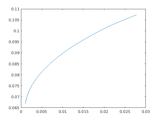
Fig. 11.1 The efficient frontier for the sample data.
Example code
Listing 11.2 demonstrates how to compute the efficient portfolios for several values of \(\alpha\).
here to download.¶#include <math.h>
#include <stdio.h>
#include "mosek.h"
#define MOSEKCALL(_r,_call) if ( (_r)==MSK_RES_OK ) (_r) = (_call)
#define LOGLEVEL 0
static void MSKAPI printstr(void *handle,
const char str[])
{
printf("%s", str);
} /* printstr */
int main(int argc, const char **argv)
{
char buf[128];
const MSKint32t n = 8;
const MSKrealt mu[] = {0.07197349, 0.15518171, 0.17535435, 0.0898094 , 0.42895777, 0.39291844, 0.32170722, 0.18378628};
// GT must have size n rows
const MSKrealt GT[][8] = {
{0.30758, 0.12146, 0.11341, 0.11327, 0.17625, 0.11973, 0.10435, 0.10638},
{0.0, 0.25042, 0.09946, 0.09164, 0.06692, 0.08706, 0.09173, 0.08506},
{0.0, 0.0, 0.19914, 0.05867, 0.06453, 0.07367, 0.06468, 0.01914},
{0.0, 0.0, 0.0, 0.20876, 0.04933, 0.03651, 0.09381, 0.07742},
{0.0, 0.0, 0.0, 0.0, 0.36096, 0.12574, 0.10157, 0.0571 },
{0.0, 0.0, 0.0, 0.0, 0.0, 0.21552, 0.05663, 0.06187},
{0.0, 0.0, 0.0, 0.0, 0.0, 0.0, 0.22514, 0.03327},
{0.0, 0.0, 0.0, 0.0, 0.0, 0.0, 0.0, 0.2202 }
};
const MSKint32t k = sizeof(GT) / (n * sizeof(MSKrealt));
const MSKrealt x0[] = {0.0, 0.0, 0.0, 0.0, 0.0, 0.0, 0.0, 0.0};
const MSKrealt w = 1.0;
const MSKrealt alphas[] = {0.0, 0.01, 0.1, 0.25, 0.30, 0.35, 0.4, 0.45, 0.5, 0.75, 1.0, 1.5, 2.0, 3.0, 10.0};
const MSKint32t numalpha = 15;
MSKrealt totalBudget;
MSKenv_t env;
MSKint32t i, j;
MSKrescodee res = MSK_RES_OK, lres;
MSKtask_t task;
MSKrealt xj;
MSKsolstae solsta;
//Offset of variables into the API variable.
MSKint32t numvar = n + 1;
MSKint32t voff_x = 0;
MSKint32t voff_s = n;
// Constraints offsets
MSKint32t numcon = 1;
MSKint32t coff_bud = 0;
/* Initial setup. */
env = NULL;
task = NULL;
/* Replace "" with NULL in production. */
MOSEKCALL(res, MSK_makeenv(&env, ""));
MOSEKCALL(res, MSK_maketask(env, 0, 0, &task));
MOSEKCALL(res, MSK_linkfunctotaskstream(task, MSK_STREAM_LOG, NULL, printstr));
// Holding variable x of length n
MOSEKCALL(res, MSK_appendvars(task, numvar));
// Setting up variable x
for (j = 0; j < n; ++j)
{
/* Optionally we can give the variables names */
sprintf(buf, "x[%d]", 1 + j);
MOSEKCALL(res, MSK_putvarname(task, voff_x + j, buf));
/* No short-selling - x^l = 0, x^u = inf */
MOSEKCALL(res, MSK_putvarbound(task, voff_x + j, MSK_BK_LO, 0.0, MSK_INFINITY));
}
sprintf(buf, "s");
MOSEKCALL(res, MSK_putvarname(task, voff_s, buf));
MOSEKCALL(res, MSK_putvarbound(task, voff_s, MSK_BK_FR, -MSK_INFINITY, MSK_INFINITY));
// One linear constraint: total budget
MOSEKCALL(res, MSK_appendcons(task, 1));
sprintf(buf, "%s", "budget");
MOSEKCALL(res, MSK_putconname(task, coff_bud, buf));
for (j = 0; j < n; ++j)
{
/* Coefficients in the first row of A */
MOSEKCALL(res, MSK_putaij(task, coff_bud, voff_x + j, 1.0));
}
totalBudget = w;
for (i = 0; i < n; ++i)
{
totalBudget += x0[i];
}
MOSEKCALL(res, MSK_putconbound(task, coff_bud, MSK_BK_FX, totalBudget, totalBudget));
// Input (gamma, GTx) in the AFE (affine expression) storage
// We build the following F and g for variables [x, s]:
// [0, 1] [0 ]
// F = [0, 0], g = [0.5]
// [GT,0] [0 ]
// We need k+2 rows
MOSEKCALL(res, MSK_appendafes(task, k + 2));
// The first affine expression is variable s (last variable, index n)
MOSEKCALL(res, MSK_putafefentry(task, 0, n, 1.0));
// The second affine expression is constant 0.5
MOSEKCALL(res, MSK_putafeg(task, 1, 0.5));
// The remaining k expressions comprise GT*x, we add them row by row
// In more realisic scenarios it would be better to extract nonzeros and input in sparse form
MSKint32t* vslice_x = (MSKint32t*) malloc(n * sizeof(MSKint32t));
for (i = 0; i < n; ++i)
{
vslice_x[i] = voff_x + i;
}
for (i = 0; i < k; ++i)
{
MOSEKCALL(res, MSK_putafefrow(task, i + 2, n, vslice_x, GT[i]));
}
free(vslice_x);
// Input the affine conic constraint (gamma, GT*x) \in QCone
// Add the quadratic domain of dimension k+1
MSKint64t rqdom;
MOSEKCALL(res, MSK_appendrquadraticconedomain(task, k + 2, &rqdom));
// Add the constraint
MOSEKCALL(res, MSK_appendaccseq(task, rqdom, k + 2, 0, NULL));
sprintf(buf, "%s", "risk");
MOSEKCALL(res, MSK_putaccname(task, 0, buf));
// Objective: maximize expected return mu^T x
for (j = 0; j < n; ++j)
{
MOSEKCALL(res, MSK_putcj(task, voff_x + j, mu[j]));
}
MOSEKCALL(res, MSK_putobjsense(task, MSK_OBJECTIVE_SENSE_MAXIMIZE));
/* Set the log level */
MOSEKCALL(res, MSK_putintparam(task, MSK_IPAR_LOG, LOGLEVEL));
printf("%-12s %-12s %-12s\n", "alpha", "exp ret", "std. dev");
for (i = 0; i < numalpha && res==MSK_RES_OK; ++i)
{
const double alpha = alphas[i];
MSKrescodee trmcode;
/* Sets the objective function coefficient for s. */
MOSEKCALL(res, MSK_putcj(task, voff_s + 0, -alpha));
MOSEKCALL(res, MSK_optimizetrm(task, &trmcode));
// Check if the interior point solution is an optimal point
MOSEKCALL(res, MSK_getsolsta(task, MSK_SOL_ITR, &solsta));
if (solsta != MSK_SOL_STA_OPTIMAL)
{
// See https://docs.mosek.com/latest/capi/accessing-solution.html about handling solution statuses.
fprintf(stderr, "Unexpected solution status: %d", solsta);
return MSK_RES_ERR_UNHANDLED_SOLUTION_STATUS;
}
if (solsta == MSK_SOL_STA_OPTIMAL)
{
double expret = 0.0,
stddev;
for (j = 0; j < n; ++j)
{
MOSEKCALL(res, MSK_getxxslice(task, MSK_SOL_ITR, voff_x + j, voff_x + j + 1, &xj));
expret += mu[j] * xj;
}
MOSEKCALL(res, MSK_getxxslice(task, MSK_SOL_ITR, voff_s + 0, voff_s + 1, &stddev));
printf("%-12.3e %-12.3e %-12.3e\n", alpha, expret, sqrt(stddev));
}
else
{
printf("An error occurred when solving for alpha=%e\n", alpha);
}
}
lres = MSK_deletetask(&task);
res = res==MSK_RES_OK ? lres : res;
lres = MSK_deleteenv(&env);
res = res==MSK_RES_OK ? lres : res;
return ( res );
}
Note that we changed the coefficient \(\alpha\) of the variable \(s\) in a loop. This way we were able to reuse the same model for all solves along the efficient frontier, simply changing the value of \(\alpha\) between the solves.
11.1.3 Factor model and efficiency
In practice it is often important to solve the portfolio problem very quickly. Therefore, in this section we discuss how to improve computational efficiency at the modeling stage.
The computational cost is of course to some extent dependent on the number of constraints and variables in the optimization problem. However, in practice a more important factor is the sparsity: the number of nonzeros used to represent the problem. Indeed it is often better to focus on the number of nonzeros in \(G\) see (11.2) and try to reduce that number by for instance changing the choice of \(G\).
In other words if the computational efficiency should be improved then it is always good idea to start with focusing at the covariance matrix. As an example assume that
where \(D\) is a positive definite diagonal matrix. Moreover, \(V\) is a matrix with \(n\) rows and \(k\) columns. Such a model for the covariance matrix is called a factor model and usually \(k\) is much smaller than \(n\). In practice \(k\) tends to be a small number independent of \(n\), say less than 100.
One possible choice for \(G\) is the Cholesky factorization of \(\Sigma\) which requires storage proportional to \(n(n+1)/2\). However, another choice is
because then
This choice requires storage proportional to \(n+kn\) which is much less than for the Cholesky choice of \(G\). Indeed assuming \(k\) is a constant storage requirements are reduced by a factor of \(n\).
The example above exploits the so-called factor structure and demonstrates that an alternative choice of \(G\) may lead to a significant reduction in the amount of storage used to represent the problem. This will in most cases also lead to a significant reduction in the solution time.
The lesson to be learned is that it is important to investigate how the covariance matrix is formed. Given this knowledge it might be possible to make a special choice for \(G\) that helps reducing the storage requirements and enhance the computational efficiency. More details about this process can be found in [And13].
Factor model in finance
Factor model structure is typical in financial context. It is common to model security returns as the sum of two components using a factor model. The first component is the linear combination of a small number of factors common among a group of securities. The second component is a residual, specific to each security. It can be written as \(R = \sum_j\beta_j F_j + \theta\), where \(R\) is a random variable representing the return of a security at a particular point in time, \(F_j\) is the random variable representing the common factor \(j\), \(\beta_j\) is the exposure of the return to factor \(j\), and \(\theta\) is the specific component.
Such a model will result in the covariance structure
where \(\Sigma_F\) is the covariance of the factors and \(\Sigma_\theta\) is the residual covariance. This structure is of the form discussed earlier with \(D = \Sigma_\theta\) and \(V = \beta P\), assuming the decomposition \(\Sigma_F = PP^T\). If the number of factors \(k\) is low and \(\Sigma_\theta\) is diagonal, we get a very sparse \(G\) that provides the storage and solution time benefits.
Example code
Here we will work with the example data of a two-factor model (\(k=2\)) built using the variables
and the factor covariance matrix is
giving
Then the matrix \(G\) would look like
This matrix is indeed very sparse.
In general, we get an \(n\times (n+k)\) size matrix this way with \(k\) full columns and an \(n\times n\) diagonal part. In order to maintain a sparse representation we do not construct the matrix \(G\) explicitly in the code but instead work with two pieces of data: the dense matrix \(G_\mathrm{factor} = \beta P\) of shape \(n\times k\) and the diagonal vector \(\theta\) of length \(n\).
Example code
In the following we demonstrate how to write code to compute the matrix \(G_\mathrm{factor}\) of the factor model. We start with the inputs
  // NOTE: Here we specify matrices as vectors (row major order) to avoid having
  // to initialize them as double(*)[] type, which is incompatible with double**.

  // Factor exposure matrix
  MSKrealt vecB[] =
  {
    0.4256, 0.1869,
    0.2413, 0.3877,
    0.2235, 0.3697,
    0.1503, 0.4612,
    1.5325, -0.2633,
    1.2741, -0.2613,
    0.6939, 0.2372,
    0.5425, 0.2116
  };
  matrix* B = vec_to_mat_r(vecB, n, 2);
  // Factor covariance matrix
  MSKrealt vecS_F[] =
  {
    0.0620, 0.0577,
    0.0577, 0.0908
  };
  matrix* S_F = vec_to_mat_r(vecS_F, 2, 2);

  // Specific risk components
  MSKrealt theta[] = {0.0720, 0.0508, 0.0377, 0.0394, 0.0663, 0.0224, 0.0417, 0.0459};
Then the matrix \(G_\mathrm{factor}\) is obtained as:
  matrix* P = cholesky(&env, S_F);
  matrix* G_factor = matrix_mul(&env, B, P);
The code for computing an optimal portfolio in the factor model is very similar to the one from the basic model in Listing 11.1 with one notable exception: we construct the expression \(G^Tx\) appearing in the conic constraint by stacking together two separate vectors \(G_\mathrm{factor}^T x\) and \(\Sigma^{1/2}_\theta x\):
  // Input (gamma, G_factor_T x, diag(sqrt(theta))*x) in the AFE (affine expression) storage
  // We need k+n+1 rows and we fill them in in three parts
  MOSEKCALL(res, MSK_appendafes(task, k + n + 1));
  // 1. The first affine expression = gamma, will be specified later
  // 2. The next k expressions comprise G_factor_T*x, we add them column by column since
  //    G_factor is stored row-wise and we transpose on the fly
  MSKint64t* afeidxs = (MSKint64t*) malloc(k * sizeof(MSKint64t));
  for (i = 0; i < k; ++i)
  {
    afeidxs[i] = i + 1;
  }
  for (i = 0; i < n; ++i)
  {
    MOSEKCALL(res, MSK_putafefcol(task, i, k, afeidxs, G_factor->m[i])); //i-th row of G_factor goes in i-th column of F
  }
  free(afeidxs);
  // 3. The remaining n rows contain sqrt(theta) on the diagonal
  for (i = 0; i < n; ++i)
  {
    MOSEKCALL(res, MSK_putafefentry(task, k + 1 + i, voff_x + i, sqrt(theta[i])));
  }
The full code is demonstrated below:
int main(int argc, const char **argv)
{
  char            buf[128];

  MSKrealt        expret  = 0.0,
                  xj;

  MSKrealt        rtemp;
  MSKenv_t        env;
  MSKint32t       i, j, *sub;
  MSKrescodee     res = MSK_RES_OK, trmcode;
  MSKtask_t       task;

  MSKint32t  n      = 8;
  MSKrealt   w      = 1.0;
  MSKrealt   mu[]   = {0.07197, 0.15518, 0.17535, 0.08981, 0.42896, 0.39292, 0.32171, 0.18379};
  MSKrealt   x0[]   = {0.0, 0.0, 0.0, 0.0, 0.0, 0.0, 0.0, 0.0};

  /* Initial setup. */
  env  = NULL;
  task = NULL;
  MOSEKCALL(res, MSK_makeenv(&env, NULL));
  MOSEKCALL(res, MSK_maketask(env, 0, 0, &task));
  MOSEKCALL(res, MSK_linkfunctotaskstream(task, MSK_STREAM_LOG, NULL, printstr));

  // NOTE: Here we specify matrices as vectors (row major order) to avoid having
  // to initialize them as double(*)[] type, which is incompatible with double**.

  // Factor exposure matrix
  MSKrealt vecB[] =
  {
    0.4256, 0.1869,
    0.2413, 0.3877,
    0.2235, 0.3697,
    0.1503, 0.4612,
    1.5325, -0.2633,
    1.2741, -0.2613,
    0.6939, 0.2372,
    0.5425, 0.2116
  };
  matrix* B = vec_to_mat_r(vecB, n, 2);
  // Factor covariance matrix
  MSKrealt vecS_F[] =
  {
    0.0620, 0.0577,
    0.0577, 0.0908
  };
  matrix* S_F = vec_to_mat_r(vecS_F, 2, 2);

  // Specific risk components
  MSKrealt theta[] = {0.0720, 0.0508, 0.0377, 0.0394, 0.0663, 0.0224, 0.0417, 0.0459};

  matrix* P = cholesky(&env, S_F);
  matrix* G_factor = matrix_mul(&env, B, P);
  matrix_free(B);
  matrix_free(S_F);
  matrix_free(P);

  MSKint32t k = G_factor->nc;
  MSKrealt gammas[] = {0.24, 0.28, 0.32, 0.36, 0.4, 0.44, 0.48};
  int num_gammas = 7;
  MSKrealt   totalBudget;

  //Offset of variables into the API variable.
  MSKint32t numvar = n;
  MSKint32t voff_x = 0;

  // Constraint offset
  MSKint32t coff_bud = 0;

  // Holding variable x of length n
  // No other auxiliary variables are needed in this formulation
  MOSEKCALL(res, MSK_appendvars(task, numvar));
  // Setting up variable x
  for (j = 0; j < n; ++j)
  {
    /* Optionally we can give the variables names */
    sprintf(buf, "x[%d]", 1 + j);
    MOSEKCALL(res, MSK_putvarname(task, voff_x + j, buf));
    /* No short-selling - x^l = 0, x^u = inf */
    MOSEKCALL(res, MSK_putvarbound(task, voff_x + j, MSK_BK_LO, 0.0, MSK_INFINITY));
  }

  // One linear constraint: total budget
  MOSEKCALL(res, MSK_appendcons(task, 1));
  sprintf(buf, "%s", "budget");
  MOSEKCALL(res, MSK_putconname(task, coff_bud, buf));
  for (j = 0; j < n; ++j)
  {
    /* Coefficients in the first row of A */
    MOSEKCALL(res, MSK_putaij(task, coff_bud, voff_x + j, 1.0));
  }
  totalBudget = w;
  for (i = 0; i < n; ++i)
  {
    totalBudget += x0[i];
  }
  MOSEKCALL(res, MSK_putconbound(task, coff_bud, MSK_BK_FX, totalBudget, totalBudget));

  // Input (gamma, G_factor_T x, diag(sqrt(theta))*x) in the AFE (affine expression) storage
  // We need k+n+1 rows and we fill them in in three parts
  MOSEKCALL(res, MSK_appendafes(task, k + n + 1));
  // 1. The first affine expression = gamma, will be specified later
  // 2. The next k expressions comprise G_factor_T*x, we add them column by column since
  //    G_factor is stored row-wise and we transpose on the fly
  MSKint64t* afeidxs = (MSKint64t*) malloc(k * sizeof(MSKint64t));
  for (i = 0; i < k; ++i)
  {
    afeidxs[i] = i + 1;
  }
  for (i = 0; i < n; ++i)
  {
    MOSEKCALL(res, MSK_putafefcol(task, i, k, afeidxs, G_factor->m[i])); //i-th row of G_factor goes in i-th column of F
  }
  free(afeidxs);
  // 3. The remaining n rows contain sqrt(theta) on the diagonal
  for (i = 0; i < n; ++i)
  {
    MOSEKCALL(res, MSK_putafefentry(task, k + 1 + i, voff_x + i, sqrt(theta[i])));
  }

  // Input the affine conic constraint (gamma, G_factor_T x, diag(sqrt(theta))*x) \in QCone
  // Add the quadratic domain of dimension k+n+1
  MSKint64t qdom;
  MOSEKCALL(res, MSK_appendquadraticconedomain(task, k + n + 1, &qdom));
  // Add the constraint
  MOSEKCALL(res, MSK_appendaccseq(task, qdom, k + n + 1, 0, NULL));
  sprintf(buf, "%s", "risk");
  MOSEKCALL(res, MSK_putaccname(task, 0, buf));

  // Objective: maximize expected return mu^T x
  for (j = 0; j < n; ++j)
  {
    MOSEKCALL(res, MSK_putcj(task, voff_x + j, mu[j]));
  }
  MOSEKCALL(res, MSK_putobjsense(task, MSK_OBJECTIVE_SENSE_MAXIMIZE));

#if 0
  /* No log output */
  MOSEKCALL(res, MSK_putintparam(task, MSK_IPAR_LOG, 0));
#endif

  for (i = 0; i < num_gammas; i++)
  {
    MSKrealt gamma = gammas[i];

    // Specify gamma in ACC
    MOSEKCALL(res, MSK_putafeg(task, 0, gamma));

#if 0
    /* Dump the problem to a human readable PTF file. */
    MOSEKCALL(res, MSK_writedata(task, "dump.ptf"));
#endif

    MOSEKCALL(res, MSK_optimizetrm(task, &trmcode));

#if 1
    /* Display the solution summary for quick inspection of results. */
    MSK_solutionsummary(task, MSK_STREAM_MSG);
#endif

// Check if the interior point solution is an optimal point
MSKsolstae solsta;
MOSEKCALL(res, MSK_getsolsta(task, MSK_SOL_ITR, &solsta));
if (solsta != MSK_SOL_STA_OPTIMAL)
{
  // See https://docs.mosek.com/latest/capi/accessing-solution.html about handling solution statuses.
  fprintf(stderr, "Unexpected solution status: %d", solsta);
  return MSK_RES_ERR_UNHANDLED_SOLUTION_STATUS;
}

    if ( res == MSK_RES_OK )
    {
      expret = 0.0;

      /* Read the x variables one by one and compute expected return. */
      /* Can also be obtained as value of the objective. */
      for (j = 0; j < n; ++j)
      {
        MOSEKCALL(res, MSK_getxxslice(task, MSK_SOL_ITR, voff_x + j, voff_x + j + 1, &xj));
        expret += mu[j] * xj;
      }

      printf("\nExpected return %e for gamma %e\n", expret, gamma);
    }
  }

  if ( task != NULL )
    MSK_deletetask(&task);

  if ( env != NULL )
    MSK_deleteenv(&env);

  matrix_free(G_factor);

  return ( 0 );
}
11.1.4 Slippage Cost
The basic Markowitz model assumes that there are no costs associated with trading the assets and that the returns of the assets are independent of the amount traded. Neither of those assumptions is usually valid in practice. Therefore, a more realistic model is
Here \(\Delta x_j\) is the change in the holding of asset \(j\) i.e.
and \(T_j(\Delta x_j)\) specifies the transaction costs when the holding of asset \(j\) is changed from its initial value. In the next two sections we show two different variants of this problem with two nonlinear cost functions \(T\).
11.1.5 Market Impact Costs
If the initial wealth is fairly small and no short selling is allowed, then the holdings will be small and the traded amount of each asset must also be small. Therefore, it is reasonable to assume that the prices of the assets are independent of the amount traded. However, if a large volume of an asset is sold or purchased, the price, and hence return, can be expected to change. This effect is called market impact costs. It is common to assume that the market impact cost for asset \(j\) can be modeled by
where \(m_j\) is a constant that is estimated in some way by the trader. See [GK00] [p. 452] for details. From the Modeling Cookbook we know that \(t \geq |z|^{3/2}\) can be modeled directly using the power cone \(\POW_3^{2/3,1/3}\):
Hence, it follows that \(\sum_{j=1}^n T_j(\Delta x_j)=\sum_{j=1}^n m_j|x_j-x_j^0|^{3/2}\) can be modeled by \(\sum_{j=1}^n m_jt_j\) under the constraints
Unfortunately this set of constraints is nonconvex due to the constraint
but in many cases the constraint may be replaced by the relaxed constraint
For instance if the universe of assets contains a risk free asset then
cannot hold for an optimal solution.
If the optimal solution has the property (11.9) then the market impact cost within the model is larger than the true market impact cost and hence money are essentially considered garbage and removed by generating transaction costs. This may happen if a portfolio with very small risk is requested because the only way to obtain a small risk is to get rid of some of the assets by generating transaction costs. We generally assume that this is not the case and hence the models (11.7) and (11.8) are equivalent.
The above observations lead to
The revised budget constraint
specifies that the initial wealth covers the investment and the transaction costs. It should be mentioned that transaction costs of the form
where \(p>1\) is a real number can be modeled with the power cone as
See the Modeling Cookbook for details.
Example code
Listing 11.5 demonstrates how to compute an optimal portfolio when market impact cost are included.
#include <math.h>
#include <stdio.h>

#include "mosek.h"

#define MOSEKCALL(_r,_call)  if ( (_r)==MSK_RES_OK ) (_r) = (_call)

static void MSKAPI printstr(void *handle,
                            const char str[])
{
  printf("%s", str);
} /* printstr */

int main(int argc, const char **argv)
{
  char            buf[128];
  const MSKint32t n       = 8;
  const MSKrealt  mu[]    = {0.07197, 0.15518, 0.17535, 0.08981, 0.42896, 0.39292, 0.32171, 0.18379};
  // GT must have size n rows
  const MSKrealt  GT[][8] = {
    {0.30758, 0.12146, 0.11341, 0.11327, 0.17625, 0.11973, 0.10435, 0.10638},
    {0.0,     0.25042, 0.09946, 0.09164, 0.06692, 0.08706, 0.09173, 0.08506},
    {0.0,     0.0,     0.19914, 0.05867, 0.06453, 0.07367, 0.06468, 0.01914},
    {0.0,     0.0,     0.0,     0.20876, 0.04933, 0.03651, 0.09381, 0.07742},
    {0.0,     0.0,     0.0,     0.0,     0.36096, 0.12574, 0.10157, 0.0571 },
    {0.0,     0.0,     0.0,     0.0,     0.0,     0.21552, 0.05663, 0.06187},
    {0.0,     0.0,     0.0,     0.0,     0.0,     0.0,     0.22514, 0.03327},
    {0.0,     0.0,     0.0,     0.0,     0.0,     0.0,     0.0,     0.2202 }
  };
  const MSKint32t k       = sizeof(GT) / (n * sizeof(MSKrealt));
  const MSKrealt  x0[]    = {0.0, 0.0, 0.0, 0.0, 0.0, 0.0, 0.0, 0.0};
  const MSKrealt  w       = 1.0;
  const MSKrealt  gamma   = 0.36;
  MSKrealt totalBudget;
  MSKint32t       i, j;

  MSKrealt* m = (MSKrealt*) malloc(n * sizeof(MSKrealt));
  for (i = 0; i < n; ++i)
  {
    m[i] = 0.01;
  }

  // Offset of variables into the API variable.
  MSKint32t numvar = 3 * n;
  MSKint32t voff_x = 0;
  MSKint32t voff_c = n;
  MSKint32t voff_z = 2 * n;

  // Offset of constraints.
  MSKint32t numcon = 2 * n + 1;
  MSKint32t coff_bud = 0;
  MSKint32t coff_abs1 = 1;
  MSKint32t coff_abs2 = 1 + n;

  double          expret,
                  stddev,
                  xj;
  MSKenv_t        env;
  MSKrescodee     res = MSK_RES_OK, trmcode;
  MSKtask_t       task;

  /* Initial setup. */
  env  = NULL;
  task = NULL;
  MOSEKCALL(res, MSK_makeenv(&env, NULL));
  MOSEKCALL(res, MSK_maketask(env, 0, 0, &task));
  MOSEKCALL(res, MSK_linkfunctotaskstream(task, MSK_STREAM_LOG, NULL, printstr));

  // Variables (vector of x, c, z)
  MOSEKCALL(res, MSK_appendvars(task, numvar));
  for (j = 0; j < n; ++j)
  {
    /* Optionally we can give the variables names */
    sprintf(buf, "x[%d]", 1 + j);
    MOSEKCALL(res, MSK_putvarname(task, voff_x + j, buf));
    sprintf(buf, "c[%d]", 1 + j);
    MOSEKCALL(res, MSK_putvarname(task, voff_c + j, buf));
    sprintf(buf, "z[%d]", 1 + j);
    MOSEKCALL(res, MSK_putvarname(task, voff_z + j, buf));
    /* Apply variable bounds (x >= 0, c and z free) */
    MOSEKCALL(res, MSK_putvarbound(task, voff_x + j, MSK_BK_LO, 0.0, MSK_INFINITY));
    MOSEKCALL(res, MSK_putvarbound(task, voff_c + j, MSK_BK_FR, -MSK_INFINITY, MSK_INFINITY));
    MOSEKCALL(res, MSK_putvarbound(task, voff_z + j, MSK_BK_FR, -MSK_INFINITY, MSK_INFINITY));
  }

  // Linear constraints
  // - Total budget
  MOSEKCALL(res, MSK_appendcons(task, 1));
  sprintf(buf, "%s", "budget");
  MOSEKCALL(res, MSK_putconname(task, coff_bud, buf));
  for (j = 0; j < n; ++j)
  {
    /* Coefficients in the first row of A */
    MOSEKCALL(res, MSK_putaij(task, coff_bud, voff_x + j, 1.0));
    MOSEKCALL(res, MSK_putaij(task, coff_bud, voff_c + j, m[j]));
  }
  totalBudget = w;
  for (i = 0; i < n; ++i)
  {
    totalBudget += x0[i];
  }
  MOSEKCALL(res, MSK_putconbound(task, coff_bud, MSK_BK_FX, totalBudget, totalBudget));

  // - Absolute value
  MOSEKCALL(res, MSK_appendcons(task, 2 * n));
  for (i = 0; i < n; ++i)
  {
    sprintf(buf, "zabs1[%d]", 1 + i);
    MOSEKCALL(res, MSK_putconname(task, coff_abs1 + i, buf));
    MOSEKCALL(res, MSK_putaij(task, coff_abs1 + i, voff_x + i, -1.0));
    MOSEKCALL(res, MSK_putaij(task, coff_abs1 + i, voff_z + i, 1.0));
    MOSEKCALL(res, MSK_putconbound(task, coff_abs1 + i, MSK_BK_LO, -x0[i], MSK_INFINITY));
    sprintf(buf, "zabs2[%d]", 1 + i);
    MOSEKCALL(res, MSK_putconname(task, coff_abs2 + i, buf));
    MOSEKCALL(res, MSK_putaij(task, coff_abs2 + i, voff_x + i, 1.0));
    MOSEKCALL(res, MSK_putaij(task, coff_abs2 + i, voff_z + i, 1.0));
    MOSEKCALL(res, MSK_putconbound(task, coff_abs2 + i, MSK_BK_LO, x0[i], MSK_INFINITY));
  }

  // ACCs
  MSKint32t aoff_q = 0;
  MSKint32t aoff_pow = k + 1;
  // - (gamma, GTx) in Q(k+1)
  // The part of F and g for variable x:
  //     [0,  0, 0]      [gamma]
  // F = [GT, 0, 0], g = [0    ]
  MOSEKCALL(res, MSK_appendafes(task, k + 1));
  MOSEKCALL(res, MSK_putafeg(task, aoff_q, gamma));
  MSKint32t* vslice_x = (MSKint32t*) malloc(n * sizeof(MSKint32t));
  for (i = 0; i < n; ++i)
  {
    vslice_x[i] = voff_x + i;
  }
  for (i = 0; i < k; ++i)
  {
    MOSEKCALL(res, MSK_putafefrow(task, aoff_q + i + 1, n, vslice_x, GT[i]));
  }
  free(vslice_x);
  MSKint64t qdom;
  MOSEKCALL(res, MSK_appendquadraticconedomain(task, k + 1, &qdom));
  MOSEKCALL(res, MSK_appendaccseq(task, qdom, k + 1, aoff_q, NULL));
  sprintf(buf, "%s", "risk");
  MOSEKCALL(res, MSK_putaccname(task, aoff_q, buf));

  // - (c_j, 1, z_j) in P3(2/3, 1/3)
  // The part of F and g for variables [c, z]:
  //     [0, I, 0]      [0]
  // F = [0, 0, I], g = [0]
  //     [0, 0, 0]      [1]
  MOSEKCALL(res, MSK_appendafes(task, 2 * n + 1));
  for (i = 0; i < n; ++i)
  {
    MOSEKCALL(res, MSK_putafefentry(task, aoff_pow + i, voff_c + i, 1.0));
    MOSEKCALL(res, MSK_putafefentry(task, aoff_pow + n + i, voff_z + i, 1.0));
  }
  MOSEKCALL(res, MSK_putafeg(task, aoff_pow + 2 * n, 1.0));
  // We use one row from F and g for both c_j and z_j, and the last row of F and g for the constant 1.
  // NOTE: Here we reuse the last AFE and the power cone n times, but we store them only once.
  MSKrealt exponents[] = {2, 1};
  MSKint64t powdom;
  MOSEKCALL(res, MSK_appendprimalpowerconedomain(task, 3, 2, exponents, &powdom));
  MSKint64t* flat_afe_list = (MSKint64t*) malloc(3 * n * sizeof(MSKint64t));
  MSKint64t* dom_list = (MSKint64t*) malloc(n * sizeof(MSKint64t));
  for (i = 0; i < n; ++i)
  {
    flat_afe_list[3 * i + 0] = aoff_pow + i;
    flat_afe_list[3 * i + 1] = aoff_pow + 2 * n;
    flat_afe_list[3 * i + 2] = aoff_pow + n + i;
    dom_list[i] = powdom;
  }
  MOSEKCALL(res, MSK_appendaccs(task, n, dom_list, 3 * n, flat_afe_list, NULL));
  free(flat_afe_list);
  free(dom_list);
  for (i = 0; i < n; ++i)
  {
    sprintf(buf, "market_impact[%d]", i);
    MOSEKCALL(res, MSK_putaccname(task, i + 1, buf));
  }

  // Objective: maximize expected return mu^T x
  for (j = 0; j < n; ++j)
  {
    MOSEKCALL(res, MSK_putcj(task, voff_x + j, mu[j]));
  }
  MOSEKCALL(res, MSK_putobjsense(task, MSK_OBJECTIVE_SENSE_MAXIMIZE));

  #if 0
    /* no log output. */
    MOSEKCALL(res, MSK_putintparam(task, MSK_IPAR_LOG, 0));
  #endif

  #if 0
    /* Dump the problem to a human readable OPF file. */
    MOSEKCALL(res, MSK_writedata(task, "dump.ptf"));
  #endif

    MOSEKCALL(res, MSK_optimizetrm(task, &trmcode));

    /* Display the solution summary for quick inspection of results. */
  #if 1
    MSK_solutionsummary(task, MSK_STREAM_MSG);
  #endif

  // Check if the interior point solution is an optimal point
  MSKsolstae solsta;
  MOSEKCALL(res, MSK_getsolsta(task, MSK_SOL_ITR, &solsta));
  if (solsta != MSK_SOL_STA_OPTIMAL)
  {
    // See https://docs.mosek.com/latest/capi/accessing-solution.html about handling solution statuses.
    fprintf(stderr, "Unexpected solution status: %d", solsta);
    return MSK_RES_ERR_UNHANDLED_SOLUTION_STATUS;
  }

  if (res == MSK_RES_OK)
  {
    expret = 0.0;
    stddev = 0.0;

    for (j = 0; j < n; ++j)
    {
      MOSEKCALL(res, MSK_getxxslice(task, MSK_SOL_ITR, voff_x + j, voff_x + j + 1, &xj));
      expret += mu[j] * xj;
    }

    printf("\nExpected return %e for gamma %e\n", expret, gamma);
  }

  MSK_deletetask(&task);
  MSK_deleteenv(&env);

  free(m);

  return (0);
}
Note that in the following part of the code:
  MOSEKCALL(res, MSK_putafeg(task, aoff_pow + 2 * n, 1.0));
  // We use one row from F and g for both c_j and z_j, and the last row of F and g for the constant 1.
  // NOTE: Here we reuse the last AFE and the power cone n times, but we store them only once.
  MSKrealt exponents[] = {2, 1};
  MSKint64t powdom;
  MOSEKCALL(res, MSK_appendprimalpowerconedomain(task, 3, 2, exponents, &powdom));
  MSKint64t* flat_afe_list = (MSKint64t*) malloc(3 * n * sizeof(MSKint64t));
  MSKint64t* dom_list = (MSKint64t*) malloc(n * sizeof(MSKint64t));
  for (i = 0; i < n; ++i)
  {
    flat_afe_list[3 * i + 0] = aoff_pow + i;
    flat_afe_list[3 * i + 1] = aoff_pow + 2 * n;
    flat_afe_list[3 * i + 2] = aoff_pow + n + i;
    dom_list[i] = powdom;
  }
  MOSEKCALL(res, MSK_appendaccs(task, n, dom_list, 3 * n, flat_afe_list, NULL));
  free(flat_afe_list);
  free(dom_list);
  for (i = 0; i < n; ++i)
  {
    sprintf(buf, "market_impact[%d]", i);
    MOSEKCALL(res, MSK_putaccname(task, i + 1, buf));
  }
we create a sequence of power cones of the form \((t_k, 1, x_k-x_k^0)\in \POW_3^{2/3,1/3}\). The power cones are determined by the sequence of exponents \((2,1)\); we create a single domain to account for that.
Moreover, note that the second coordinate of all these affine conic constraints is the same affine expression equal to \(1\), and we use the feature that allows us to define this affine expression only once (as AFE number aoff_pow + 2 * n) and reuse it in all the ACCs.
11.1.6 Transaction Costs
Now assume there is a cost associated with trading asset \(j\) given by
Hence, whenever asset \(j\) is traded we pay a fixed setup cost \(f_j\) and a variable cost of \(g_j\) per unit traded. Given the assumptions about transaction costs in this section problem (11.6) may be formulated as
(11.11)¶\[\begin{split}\begin{array}{lrcll} \mbox{maximize} & \mu^T x & & &\\ \mbox{subject to} & e^T x + f^Ty + g^T z & = & w + e^T x^0, &\\ & (\gamma,G^T x) & \in & \Q^{k+1}, & \\ & z_j & \geq & x_j - x_j^0, & j=1,\ldots,n,\\ & z_j & \geq & x_j^0 - x_j, & j=1,\ldots,n,\\ & z_j & \leq & U_j y_j, & j=1,\ldots,n,\\ & y_j & \in & \{0,1\}, & j=1,\ldots,n, \\ & x & \geq & 0. & \end{array}\end{split}\]
First observe that
We choose \(U_j\) as some a priori upper bound on the amount of trading in asset \(j\) and therefore if \(z_j>0\) then \(y_j = 1\) has to be the case. This implies that the transaction cost for asset \(j\) is given by
Example code
The following example code demonstrates how to compute an optimal portfolio when transaction costs are included.
#include <math.h>
#include <stdio.h>

#include "mosek.h"

#define MOSEKCALL(_r,_call)  if ( (_r)==MSK_RES_OK ) (_r) = (_call)

static void MSKAPI printstr(void *handle,
                            const char str[])
{
  printf("%s", str);
} /* printstr */

int main(int argc, const char **argv)
{
  char            buf[128];
  const MSKint32t n       = 8;
  const MSKrealt  mu[]    = {0.07197, 0.15518, 0.17535, 0.08981, 0.42896, 0.39292, 0.32171, 0.18379};
  // GT must have size n rows
  const MSKrealt  GT[][8] = {
    {0.30758, 0.12146, 0.11341, 0.11327, 0.17625, 0.11973, 0.10435, 0.10638},
    {0.0,     0.25042, 0.09946, 0.09164, 0.06692, 0.08706, 0.09173, 0.08506},
    {0.0,     0.0,     0.19914, 0.05867, 0.06453, 0.07367, 0.06468, 0.01914},
    {0.0,     0.0,     0.0,     0.20876, 0.04933, 0.03651, 0.09381, 0.07742},
    {0.0,     0.0,     0.0,     0.0,     0.36096, 0.12574, 0.10157, 0.0571 },
    {0.0,     0.0,     0.0,     0.0,     0.0,     0.21552, 0.05663, 0.06187},
    {0.0,     0.0,     0.0,     0.0,     0.0,     0.0,     0.22514, 0.03327},
    {0.0,     0.0,     0.0,     0.0,     0.0,     0.0,     0.0,     0.2202 }
  };
  const MSKint32t k       = sizeof(GT) / (n * sizeof(MSKrealt));
  const MSKrealt  x0[]    = {0.0, 0.0, 0.0, 0.0, 0.0, 0.0, 0.0, 0.0};
  const MSKrealt  w       = 1.0;
  const MSKrealt  gamma   = 0.36;

  MSKint32t       i, j;
  MSKrealt* f = (MSKrealt*) malloc(n * sizeof(MSKrealt));
  MSKrealt* g = (MSKrealt*) malloc(n * sizeof(MSKrealt));
  for (i = 0; i < n; ++i)
  {
    f[i] = 0.01;
    g[i] = 0.001;
  }

  // Offset of variables.
  MSKint32t numvar = 3 * n;
  MSKint32t voff_x = 0;
  MSKint32t voff_z = n;
  MSKint32t voff_y = 2 * n;

  // Offset of constraints.
  MSKint32t numcon = 3 * n + 1;
  MSKint32t coff_bud = 0;
  MSKint32t coff_abs1 = 1;
  MSKint32t coff_abs2 = 1 + n;
  MSKint32t coff_swi = 1 + 2 * n;

  double          expret,
                  xj;
  MSKenv_t        env;
  MSKrescodee     res = MSK_RES_OK, trmcode;
  MSKtask_t       task;

  /* Initial setup. */
  env  = NULL;
  task = NULL;
  MOSEKCALL(res, MSK_makeenv(&env, NULL));
  MOSEKCALL(res, MSK_maketask(env, 0, 0, &task));
  MOSEKCALL(res, MSK_linkfunctotaskstream(task, MSK_STREAM_LOG, NULL, printstr));

  // Variables (vector of x, z, y)
  MOSEKCALL(res, MSK_appendvars(task, numvar));
  for (j = 0; j < n; ++j)
  {
    /* Optionally we can give the variables names */
    sprintf(buf, "x[%d]", 1 + j);
    MOSEKCALL(res, MSK_putvarname(task, voff_x + j, buf));
    sprintf(buf, "z[%d]", 1 + j);
    MOSEKCALL(res, MSK_putvarname(task, voff_z + j, buf));
    sprintf(buf, "y[%d]", 1 + j);
    MOSEKCALL(res, MSK_putvarname(task, voff_y + j, buf));
    /* Apply variable bounds (x >= 0, z free, y binary) */
    MOSEKCALL(res, MSK_putvarbound(task, voff_x + j, MSK_BK_LO, 0.0, MSK_INFINITY));
    MOSEKCALL(res, MSK_putvarbound(task, voff_z + j, MSK_BK_FR, -MSK_INFINITY, MSK_INFINITY));
    MOSEKCALL(res, MSK_putvarbound(task, voff_y + j, MSK_BK_RA, 0.0, 1.0));
    MOSEKCALL(res, MSK_putvartype(task, voff_y + j, MSK_VAR_TYPE_INT));
  }

  // Linear constraints
  // - Total budget
  MOSEKCALL(res, MSK_appendcons(task, 1));
  sprintf(buf, "%s", "budget");
  MOSEKCALL(res, MSK_putconname(task, coff_bud, buf));
  for (j = 0; j < n; ++j)
  {
    /* Coefficients in the first row of A */
    MOSEKCALL(res, MSK_putaij(task, coff_bud, voff_x + j, 1.0));
    MOSEKCALL(res, MSK_putaij(task, coff_bud, voff_z + j, g[j]));
    MOSEKCALL(res, MSK_putaij(task, coff_bud, voff_y + j, f[j]));
  }
  MSKrealt U = w;
  for (i = 0; i < n; ++i)
  {
    U += x0[i];
  }
  MOSEKCALL(res, MSK_putconbound(task, coff_bud, MSK_BK_FX, U, U));

  // - Absolute value
  MOSEKCALL(res, MSK_appendcons(task, 2 * n));
  for (i = 0; i < n; ++i)
  {
    sprintf(buf, "zabs1[%d]", 1 + i);
    MOSEKCALL(res, MSK_putconname(task, coff_abs1 + i, buf));
    MOSEKCALL(res, MSK_putaij(task, coff_abs1 + i, voff_x + i, -1.0));
    MOSEKCALL(res, MSK_putaij(task, coff_abs1 + i, voff_z + i, 1.0));
    MOSEKCALL(res, MSK_putconbound(task, coff_abs1 + i, MSK_BK_LO, -x0[i], MSK_INFINITY));
    sprintf(buf, "zabs2[%d]", 1 + i);
    MOSEKCALL(res, MSK_putconname(task, coff_abs2 + i, buf));
    MOSEKCALL(res, MSK_putaij(task, coff_abs2 + i, voff_x + i, 1.0));
    MOSEKCALL(res, MSK_putaij(task, coff_abs2 + i, voff_z + i, 1.0));
    MOSEKCALL(res, MSK_putconbound(task, coff_abs2 + i, MSK_BK_LO, x0[i], MSK_INFINITY));
  }

  // - Switch
  MOSEKCALL(res, MSK_appendcons(task, n));
  for (i = 0; i < n; ++i)
  {
    sprintf(buf, "switch[%d]", 1 + i);
    MOSEKCALL(res, MSK_putconname(task, coff_swi + i, buf));
    MOSEKCALL(res, MSK_putaij(task, coff_swi + i, voff_z + i, 1.0));
    MOSEKCALL(res, MSK_putaij(task, coff_swi + i, voff_y + i, -U));
    MOSEKCALL(res, MSK_putconbound(task, coff_swi + i, MSK_BK_UP, -MSK_INFINITY, 0.0));
  }

  // ACCs
  MSKint32t aoff_q = 0;
  // - (gamma, GTx) in Q(k+1)
  // The part of F and g for variable x:
  //     [0,  0, 0]      [gamma]
  // F = [GT, 0, 0], g = [0    ]
  MOSEKCALL(res, MSK_appendafes(task, k + 1));
  MOSEKCALL(res, MSK_putafeg(task, aoff_q, gamma));
  MSKint32t* vslice_x = (MSKint32t*) malloc(n * sizeof(MSKint32t));
  for (i = 0; i < n; ++i)
  {
    vslice_x[i] = voff_x + i;
  }
  for (i = 0; i < k; ++i)
  {
    MOSEKCALL(res, MSK_putafefrow(task, aoff_q + i + 1, n, vslice_x, GT[i]));
  }
  free(vslice_x);
  MSKint64t qdom;
  MOSEKCALL(res, MSK_appendquadraticconedomain(task, k + 1, &qdom));
  MOSEKCALL(res, MSK_appendaccseq(task, qdom, k + 1, aoff_q, NULL));
  sprintf(buf, "%s", "risk");
  MOSEKCALL(res, MSK_putaccname(task, aoff_q, buf));

  // Objective: maximize expected return mu^T x
  for (j = 0; j < n; ++j)
  {
    MOSEKCALL(res, MSK_putcj(task, voff_x + j, mu[j]));
  }
  MOSEKCALL(res, MSK_putobjsense(task, MSK_OBJECTIVE_SENSE_MAXIMIZE));

#if 0
  /* no log output. */
  MOSEKCALL(res, MSK_putintparam(task, MSK_IPAR_LOG, 0));
#endif

#if 0
  /* Dump the problem to a human readable OPF file. */
  MOSEKCALL(res, MSK_writedata(task, "dump.ptf"));
#endif

  MOSEKCALL(res, MSK_optimizetrm(task, &trmcode));

#if 1
  /* Display the solution summary for quick inspection of results. */
  MSK_solutionsummary(task, MSK_STREAM_MSG);
#endif

// Check if the interior point solution is an optimal point
MSKsolstae solsta;
MOSEKCALL(res, MSK_getsolsta(task, MSK_SOL_ITG, &solsta));
if (solsta != MSK_SOL_STA_INTEGER_OPTIMAL)
{
  // See https://docs.mosek.com/latest/capi/accessing-solution.html about handling solution statuses.
  fprintf(stderr, "Unexpected solution status: %d", solsta);
  return MSK_RES_ERR_UNHANDLED_SOLUTION_STATUS;
}


  if (res == MSK_RES_OK)
  {
    expret = 0.0;

    for (j = 0; j < n; ++j)
    {
      MOSEKCALL(res, MSK_getxxslice(task, MSK_SOL_ITG, voff_x + j, voff_x + j + 1, &xj));
      expret += mu[j] * xj;
    }

    printf("\nExpected return %e for gamma %e\n", expret, gamma);
  }

  MSK_deletetask(&task);
  MSK_deleteenv(&env);

  free(f);
  free(g);

  return (0);
}
11.1.7 Cardinality constraints
Another method to reduce costs involved with processing transactions is to only change positions in a small number of assets. In other words, at most \(K\) of the differences \(|\Delta x_j|=|x_j - x_j^0|\) are allowed to be non-zero, where \(K\) is (much) smaller than the total number of assets \(n\).
This type of constraint can be again modeled by introducing a binary variable \(y_j\) which indicates if \(\Delta x_j\neq 0\) and bounding the sum of \(y_j\). The basic Markowitz model then gets updated as follows:
(11.12)¶\[\begin{split}\begin{array}{lrcll} \mbox{maximize} & \mu^T x & & &\\ \mbox{subject to} & e^T x & = & w + e^T x^0, &\\ & (\gamma,G^T x) & \in & \Q^{k+1}, & \\ & z_j & \geq & x_j - x_j^0, & j=1,\ldots,n,\\ & z_j & \geq & x_j^0 - x_j, & j=1,\ldots,n,\\ & z_j & \leq & U_j y_j, & j=1,\ldots,n,\\ & y_j & \in & \{0,1\}, & j=1,\ldots,n, \\ & e^T y & \leq & K, & \\ & x & \geq & 0, & \end{array}\end{split}\]
were \(U_j\) is some a priori chosen upper bound on the amount of trading in asset \(j\).
Example code
The following example code demonstrates how to compute an optimal portfolio with cardinality bounds.
MSKrescodee markowitz_with_card(const int        n,
                                const int        k,
                                const double     x0[],
                                const double     w,
                                const double     gamma,
                                const double     mu[],
                                const double     GT[][8],
                                const int        K,
                                      double     *xx)
{

  // Offset of variables.
  MSKint32t numvar = 3 * n;
  MSKint32t voff_x = 0;
  MSKint32t voff_z = n;
  MSKint32t voff_y = 2 * n;

  // Offset of constraints.
  MSKint32t numcon = 3 * n + 2;
  MSKint32t coff_bud = 0;
  MSKint32t coff_abs1 = 1;
  MSKint32t coff_abs2 = 1 + n;
  MSKint32t coff_swi = 1 + 2 * n;
  MSKint32t coff_card = 1 + 3 * n;

  char            buf[128];
  MSKenv_t        env;
  MSKint32t       i, j;
  MSKrescodee     res = MSK_RES_OK, trmcode;
  MSKtask_t       task;

  /* Initial setup. */
  env  = NULL;
  task = NULL;
  MOSEKCALL(res, MSK_makeenv(&env, NULL));
  MOSEKCALL(res, MSK_maketask(env, 0, 0, &task));
  MOSEKCALL(res, MSK_linkfunctotaskstream(task, MSK_STREAM_LOG, NULL, printstr));

  // Variables (vector of x, z, y)
  MOSEKCALL(res, MSK_appendvars(task, numvar));
  for (j = 0; j < n; ++j)
  {
    /* Optionally we can give the variables names */
    sprintf(buf, "x[%d]", 1 + j);
    MOSEKCALL(res, MSK_putvarname(task, voff_x + j, buf));
    sprintf(buf, "z[%d]", 1 + j);
    MOSEKCALL(res, MSK_putvarname(task, voff_z + j, buf));
    sprintf(buf, "y[%d]", 1 + j);
    MOSEKCALL(res, MSK_putvarname(task, voff_y + j, buf));
    /* Apply variable bounds (x >= 0, z free, y binary) */
    MOSEKCALL(res, MSK_putvarbound(task, voff_x + j, MSK_BK_LO, 0.0, MSK_INFINITY));
    MOSEKCALL(res, MSK_putvarbound(task, voff_z + j, MSK_BK_FR, -MSK_INFINITY, MSK_INFINITY));
    MOSEKCALL(res, MSK_putvarbound(task, voff_y + j, MSK_BK_RA, 0.0, 1.0));
    MOSEKCALL(res, MSK_putvartype(task, voff_y + j, MSK_VAR_TYPE_INT));
  }

  // Linear constraints
  // - Total budget
  MOSEKCALL(res, MSK_appendcons(task, 1));
  sprintf(buf, "%s", "budget");
  MOSEKCALL(res, MSK_putconname(task, coff_bud, buf));
  for (j = 0; j < n; ++j)
  {
    /* Coefficients in the first row of A */
    MOSEKCALL(res, MSK_putaij(task, coff_bud, voff_x + j, 1.0));
  }
  MSKrealt U = w;
  for (i = 0; i < n; ++i)
  {
    U += x0[i];
  }
  MOSEKCALL(res, MSK_putconbound(task, coff_bud, MSK_BK_FX, U, U));

  // - Absolute value
  MOSEKCALL(res, MSK_appendcons(task, 2 * n));
  for (i = 0; i < n; ++i)
  {
    sprintf(buf, "zabs1[%d]", 1 + i);
    MOSEKCALL(res, MSK_putconname(task, coff_abs1 + i, buf));
    MOSEKCALL(res, MSK_putaij(task, coff_abs1 + i, voff_x + i, -1.0));
    MOSEKCALL(res, MSK_putaij(task, coff_abs1 + i, voff_z + i, 1.0));
    MOSEKCALL(res, MSK_putconbound(task, coff_abs1 + i, MSK_BK_LO, -x0[i], MSK_INFINITY));
    sprintf(buf, "zabs2[%d]", 1 + i);
    MOSEKCALL(res, MSK_putconname(task, coff_abs2 + i, buf));
    MOSEKCALL(res, MSK_putaij(task, coff_abs2 + i, voff_x + i, 1.0));
    MOSEKCALL(res, MSK_putaij(task, coff_abs2 + i, voff_z + i, 1.0));
    MOSEKCALL(res, MSK_putconbound(task, coff_abs2 + i, MSK_BK_LO, x0[i], MSK_INFINITY));
  }

  // - Switch
  MOSEKCALL(res, MSK_appendcons(task, n));
  for (i = 0; i < n; ++i)
  {
    sprintf(buf, "switch[%d]", 1 + i);
    MOSEKCALL(res, MSK_putconname(task, coff_swi + i, buf));
    MOSEKCALL(res, MSK_putaij(task, coff_swi + i, voff_z + i, 1.0));
    MOSEKCALL(res, MSK_putaij(task, coff_swi + i, voff_y + i, -U));
    MOSEKCALL(res, MSK_putconbound(task, coff_swi + i, MSK_BK_UP, -MSK_INFINITY, 0.0));
  }

  // - Cardinality
  MOSEKCALL(res, MSK_appendcons(task, 1));
  sprintf(buf, "cardinality");
  MOSEKCALL(res, MSK_putconname(task, coff_card, buf));
  for (i = 0; i < n; ++i)
  {
    MOSEKCALL(res, MSK_putaij(task, coff_card, voff_y + i, 1.0));
    MOSEKCALL(res, MSK_putconbound(task, coff_card, MSK_BK_UP, -MSK_INFINITY, K));
  }

  // ACCs
  MSKint32t aoff_q = 0;
  // - (gamma, GTx) in Q(k+1)
  // The part of F and g for variable x:
  //     [0,  0, 0]      [gamma]
  // F = [GT, 0, 0], g = [0    ]
  MOSEKCALL(res, MSK_appendafes(task, k + 1));
  MOSEKCALL(res, MSK_putafeg(task, aoff_q, gamma));
  MSKint32t* vslice_x = (MSKint32t*) malloc(n * sizeof(MSKint32t));
  for (i = 0; i < n; ++i)
  {
    vslice_x[i] = voff_x + i;
  }
  for (i = 0; i < k; ++i)
  {
    MOSEKCALL(res, MSK_putafefrow(task, aoff_q + i + 1, n, vslice_x, GT[i]));
  }
  free(vslice_x);
  MSKint64t qdom;
  MOSEKCALL(res, MSK_appendquadraticconedomain(task, k + 1, &qdom));
  MOSEKCALL(res, MSK_appendaccseq(task, qdom, k + 1, aoff_q, NULL));
  sprintf(buf, "%s", "risk");
  MOSEKCALL(res, MSK_putaccname(task, aoff_q, buf));

  // Objective: maximize expected return mu^T x
  for (j = 0; j < n; ++j)
  {
    MOSEKCALL(res, MSK_putcj(task, voff_x + j, mu[j]));
  }
  MOSEKCALL(res, MSK_putobjsense(task, MSK_OBJECTIVE_SENSE_MAXIMIZE));

#if 0
  /* no log output. */
  MOSEKCALL(res, MSK_putintparam(task, MSK_IPAR_LOG, 0));
#endif

#if 0
  /* Dump the problem to a human readable OPF file. */
  MOSEKCALL(res, MSK_writedata(task, "dump.ptf"));
#endif

  MOSEKCALL(res, MSK_optimizetrm(task, &trmcode));

#if 1
  /* Display the solution summary for quick inspection of results. */
  MSK_solutionsummary(task, MSK_STREAM_MSG);
#endif

// Check if the interior point solution is an optimal point
MSKsolstae solsta;
MOSEKCALL(res, MSK_getsolsta(task, MSK_SOL_ITG, &solsta));
if (solsta != MSK_SOL_STA_INTEGER_OPTIMAL)
{
  // See https://docs.mosek.com/latest/capi/accessing-solution.html about handling solution statuses.
  fprintf(stderr, "Unexpected solution status: %d", solsta);
  return MSK_RES_ERR_UNHANDLED_SOLUTION_STATUS;
}

  if (res == MSK_RES_OK)
    MOSEKCALL(res, MSK_getxxslice(task, MSK_SOL_ITG, voff_x, voff_x + n, xx));

  MSK_deletetask(&task);
  MSK_deleteenv(&env);

  return res;
}
If we solve our running example with \(K=1,\dots,n\) then we get the following solutions, with increasing expected returns:
Bound 1   Solution: 0.0000e+00   0.0000e+00   1.0000e+00   0.0000e+00   0.0000e+00   0.0000e+00   0.0000e+00   0.0000e+00
Bound 2   Solution: 0.0000e+00   0.0000e+00   3.5691e-01   0.0000e+00   0.0000e+00   6.4309e-01   -0.0000e+00  0.0000e+00
Bound 3   Solution: 0.0000e+00   0.0000e+00   1.9258e-01   0.0000e+00   0.0000e+00   5.4592e-01   2.6150e-01   0.0000e+00
Bound 4   Solution: 0.0000e+00   0.0000e+00   2.0391e-01   0.0000e+00   6.7098e-02   4.9181e-01   2.3718e-01   0.0000e+00
Bound 5   Solution: 0.0000e+00   3.1970e-02   1.7028e-01   0.0000e+00   7.0741e-02   4.9551e-01   2.3150e-01   0.0000e+00
Bound 6   Solution: 0.0000e+00   3.1970e-02   1.7028e-01   0.0000e+00   7.0740e-02   4.9551e-01   2.3150e-01   0.0000e+00
Bound 7   Solution: 0.0000e+00   3.1970e-02   1.7028e-01   0.0000e+00   7.0740e-02   4.9551e-01   2.3150e-01   0.0000e+00
Bound 8   Solution: 1.9557e-10   2.6992e-02   1.6706e-01   2.9676e-10   7.1245e-02   4.9559e-01   2.2943e-01   9.6905e-03