11.3 Robust linear Optimization

In most linear optimization examples discussed in this manual it is implicitly assumed that the problem data, such as $c$ and $A$, is known with certainty. However, in practice this is seldom the case, e.g. the data may just be roughly estimated, affected by measurement errors or be affected by random events.

In this section a robust linear optimization methodology is presented which removes the assumption that the problem data is known exactly. Rather it is assumed that the data belongs to some set, i.e. a box or an ellipsoid.

The computations are performed using the MOSEK optimization toolbox for MATLAB but could equally well have been implemented using the MOSEK API.

This section is co-authored with A. Ben-Tal and A. Nemirovski. For further information about robust linear optimization consult [BTN00], [BenTalN01].

11.3.1 Introductory Example

Consider the following toy-sized linear optimization problem: A company produces two kinds of drugs, DrugI and DrugII, containing a specific active agent A, which is extracted from a raw materials that should be purchased on the market. The drug production data are as follows:

Selling price $ per 1000 packs	6200	6900
Content of agent A gm per 100 packs	0.500	0.600
Production expenses
$ per 1000 packs
Manpower, hours	90.0	100.0
Equipment, hours	40.0	50.0
Operational cost, $	700	800

There are two kinds of raw materials, RawI and RawII, which can be used as sources of the active agent. The related data is as follows:

Raw material	Purchasing price,	Content of agent A,
RawI	100.00	0.01
RawII	199.90	0.02

Finally, the monthly resources dedicated to producing the drugs are as follows:

Budget,`	Manpower	Equipment	Capacity of raw materials
100000	2000	800	1000

The problem is to find the production plan which maximizes the profit of the company, i.e. minimize the purchasing and operational costs

$$100\cdot \mathtt{RawI}+199.90\cdot \mathtt{RawII}+700\cdot \mathtt{DrugI}+800\cdot \mathtt{DrugII}$$

and maximize the income

$$6200\cdot \mathtt{DrugI}+6900\cdot \mathtt{DrugII}$$

The problem can be stated as the following linear programming program:

Minimize

(11.21)$$-\{100\cdot \mathtt{RawI}+199.90\cdot \mathtt{RawII}+700\cdot \mathtt{DrugI}+800\cdot \mathtt{DrugII}\}+\{6200\cdot \mathtt{DrugI}+6900\cdot \mathtt{DrugII}\}$$

subject to

$$\begin{array}{r}\begin{array}{rcll}0.01\cdot \mathtt{RawI}+0.02\cdot \mathtt{RawII}-0.500\cdot \mathtt{DrugI}-0.600\cdot \mathtt{DrugII}& \ge & 0& (a)\\ \mathtt{RawI}+\mathtt{RawII}& \le & 1000& (b)\\ 90.0\cdot \mathtt{DrugI}+100.0\cdot \mathtt{DrugII}& \le & 2000& (c)\\ 40.0\cdot \mathtt{DrugI}+50.0\cdot \mathtt{DrugII}& \le & 800& (d)\\ 100.0\cdot \mathtt{RawI}+199.90\cdot \mathtt{RawII}+700\cdot \mathtt{DrugI}+800\cdot \mathtt{DrugII}& \le & 100000& (d)\\ \mathtt{RawI},\mathtt{RawII},\mathtt{DrugI},\mathtt{DrugII}& \ge & 0& (e)\end{array}\end{array}$$

where the variables are the amounts RawI, RawII (in kg) of raw materials to be purchased and the amounts DrugI, DrugII (in 1000 of packs) of drugs to be produced. The objective (11.21) denotes the profit to be maximized, and the inequalities can be interpreted as follows:

• Balance of the active agent.

• Storage restriction.

• Manpower restriction.

• Equipment restriction.

• Ducget restriction.

Listing 11.13 is the MATLAB script which specifies the problem and solves it using the MOSEK optimization toolbox:

Listing 11.13 Script rlo1.m. Click here to download.

function rlo1()

prob.c   = [-100;-199.9;6200-700;6900-800];
prob.a   = sparse([0.01,0.02,-0.500,-0.600;1,1,0,0;
                   0,0,90.0,100.0;0,0,40.0,50.0;100.0,199.9,700,800]);
prob.blc = [0;-inf;-inf;-inf;-inf];
prob.buc = [inf;1000;2000;800;100000];
prob.blx = [0;0;0;0];
prob.bux = [inf;inf;inf;inf];
[r,res]  = mosekopt('maximize',prob);
xx       = res.sol.itr.xx;
RawI     = xx(1);
RawII    = xx(2);
DrugI    = xx(3);
DrugII   = xx(4);

disp(sprintf('*** Optimal value: %8.3f',prob.c'*xx));
disp('*** Optimal solution:');
disp(sprintf('RawI:   %8.3f',RawI));
disp(sprintf('RawII:  %8.3f',RawII));
disp(sprintf('DrugI:  %8.3f',DrugI));
disp(sprintf('DrugII: %8.3f',DrugII));

When executing this script, the following is displayed:

Listing 11.14 Output of script rlo1.m

*** Optimal value: 8819.658
*** Optimal solution:
RawI:     0.000
RawII:  438.789
DrugI:   17.552
DrugII:   0.000

We see that the optimal solution promises the company a modest but quite respectful profit of 8.8%. Please note that at the optimal solution the balance constraint is active: the production process utilizes the full amount of the active agent contained in the raw materials.

11.3.2 Data Uncertainty and its Consequences.

Please note that not all problem data can be regarded as absolutely reliable; e.g. one can hardly believe that the contents of the active agent in the raw materials are exactly the nominal data $0.01$ gm/kg for RawI and $0.02$ gm/kg for RawII. In reality, these contents definitely vary around the indicated values. A natural assumption here is that the actual contents of the active agent $a_i$ in RawI and $a_{II}$ in RawII are realizations of random variables somehow distributed around the nominal contents $a_i^{\text{n}}=0.01$ and $a_{II}^{\text{n}}=0.02$. To be more specific, assume that $a_i$ drifts in the $0.5\mathrm{\%}$ margin of $a_i^{\text{n}}$, i.e. it takes with probability 0.5 the values from the interval $a_i^{\text{n}}(1\pm 0.005)=a_i^{\text{n}}\{0.00995;0.01005\}$. Similarly, assume that $a_{II}$ drifts in the $2\mathrm{\%}$ margin of $a_{II}^{\text{n}}$, taking with probabilities $0.5$ the values $a_{II}^{\text{n}}(1\pm 0.02)=a_i^{\text{n}}\{0.0196;0.0204\}$. How do the perturbations of the contents of the active agent affect the production process?

The optimal solution prescribes to purchase 438.8 kg of RawII and to produce 17552 packs of DrugI. With the above random fluctuations in the content of the active agent in RawII, this production plan, with probability 0.5, will be infeasible – with this probability, the actual content of the active agent in the raw materials will be less than required to produce the planned amount of DrugI. For the sake of simplicity, assume that this difficulty is resolved in the simplest way: when the actual content of the active agent in the raw materials is insufficient, the output of the drug is reduced accordingly. With this policy, the actual production of DrugI becomes a random variable which takes, with probabilities 0.5, the nominal value of 17552 packs and the 2% less value of 17201 packs. These 2% fluctuations in the production affect the profit as well; the latter becomes a random variable taking, with probabilities 0.5, the nominal value 8,820 and the 21% less value 6,929. The expected profit is 7,843, which is by 11% less than the nominal profit 8,820 promised by the optimal solution of the problem.

We see that in our toy example that small (and in reality unavoidable) perturbations of the data may make the optimal solution infeasible, and a straightforward adjustment to the actual solution values may heavily affect the solution quality.

It turns out that the outlined phenomenon is found in many linear programs of practical origin. Usually, in these programs at least part of the data is not known exactly and can vary around its nominal values, and these data perturbations can make the nominal optimal solution – the one corresponding to the nominal data – infeasible. It turns out that the consequences of data uncertainty can be much more severe than in our toy example. The analysis of linear optimization problems from the NETLIB collection [1] reported in [BTN00] demonstrates that for 13 of 94 NETLIB problems, already 0.01% perturbations of “clearly uncertain” data can make the nominal optimal solution severely infeasible: with these perturbations, the solution, with a non-negligible probability, violates some of the constraints by 50% and more. It should be added that in the general case, in contrast to the toy example we have considered, there is no evident way to adjust the optimal solution by a small modification to the actual values of the data. Moreover there are cases when such an adjustment is impossible — in order to become feasible for the perturbed data, the nominal optimal solution should be completely reshaped.

11.3.3 Robust Linear Optimization Methodology

A natural approach to handling data uncertainty in optimization is offered by the Robust Optimization Methodology which, as applied to linear optimization, is as follows.

11.3.3.1 Uncertain Linear Programs and their Robust Counterparts.

Consider a linear optimization problem

(11.22)$$\begin{array}{r}\begin{array}{lccccc}\text{minimize}& & & c^{T}x& & \\ \text{subject to}& l_c& \le & Ax& \le & u_c,\\ & l_x& \le & x& \le & u_x,\end{array}\end{array}$$

with the data $(c,A,l_c,u_c,l_x,u_x)$, and assume that this data is not known exactly; all we know is that the data varies in a given uncertainty set $\mathcal{U}$. The simplest example is the one of interval uncertainty, where every data entry can run through a given interval:

(11.23)$$\begin{array}{r}\begin{array}{rcl}\mathcal{U}& =& \{(c,A,l_c,u_c,l_x,u_x):\\ & & (c^{\text{n}}-dc,A^{\text{n}}-dA,l_c^{\text{n}}-d{l}_c,u_c^{\text{n}}-d{u}_c,l_x^{\text{n}}-d{l}_x,u_x^{\text{n}}-d{u}_x)\le (c,A,l_c,u_c,l_x,u_x)\\ & & \le (c^{\text{n}}+dc,A^{\text{n}}+dA,l_c^{\text{n}}+d{l}_c,u_c^{\text{n}}+d{u}_c,l_x^{\text{n}}+d{l}_x,u_x^{\text{n}}+d{u}_x)\}.\end{array}\end{array}$$

Here

$$(c^{\text{n}},A^{\text{n}},l_c^{\text{n}},u_c^{\text{n}},l_x^{\text{n}},u_x^{\text{n}})$$

is the nominal data,

$$dc,dA,d{l}_c,d{u}_c,d{l}_x,d{u}_x\ge 0$$

is the data perturbation bounds. Please note that some of the entries in the data perturbation bounds can be zero, meaning that the corresponding data entries are certain (the expected values equals the actual values).

• The family of instances (11.22) with data running through a given uncertainty set $\mathcal{U}$ is called an uncertain linear optimization problem.

• Vector $x$ is called a robust feasible solution to an uncertain linear optimization problem, if it remains feasible for all realizations of the data from the uncertainty set, i.e. if

  $$l_c\le Ax\le u_c,l_x\le x\le u_x$$

for all

$$(c,A,l_c,u_c,l_x,u_x)\in \mathcal{U}.$$

• If for some value $t$ we have $c^{T}x\le t$ for all realizations of the objective from the uncertainty set, we say that robust value of the objective at $x$ does not exceed $t$.

The Robust Optimization methodology proposes to associate with an uncertain linear program its robust counterpart (RC) which is the problem of minimizing the robust optimal value over the set of all robust feasible solutions, i.e. the problem

(11.24)$$\underset{t,x}{min}\{t:c^{T}x\le t,l_c\le Ax\le u_c,l_x\le x\le u_x\mathrm{\forall }(c,A,l_c,u_c,l_x,u_x)\in \mathcal{U}\}.$$

The optimal solution to (11.24) is treated as the uncertainty-immuned solution to the original uncertain linear programming program.

11.3.3.2 Robust Counterpart of an Uncertain Linear Optimization Problem with Interval Uncertainty

In general, the RC (11.24) of an uncertain linear optimization problem is not a linear optimization problem since (11.24) has infinitely many linear constraints. There are, however, cases when (11.24) can be rewritten equivalently as a linear programming program; in particular, this is the case for interval uncertainty (11.23). Specifically, in the case of (11.23), the robust counterpart of uncertain linear program is equivalent to the following linear program in variables $x,y,t$:

(11.25)$$\begin{array}{r}\begin{array}{lcccccl}\text{minimize}& & & t& & & \\ \text{subject to}& & & (c^{\text{n}}{)}^{T}x+(dc{)}^{T}y-t& \le & 0,& (a)\\ & l_c^{\text{n}}+d{l}_c& \le & (A^{\text{n}})x-(dA)y,& & & (b)\\ & & & (A^{\text{n}})x+(dA)y& \le & u_c^{\text{n}}-d{u}_c,& (c)\\ & 0& \le & x+y,& & & (d)\\ & 0& \le & -x+y,& & & (e)\\ & l_x^{\text{n}}+d{l}_x& \le & x& \le & u_x^{\text{n}}-d{u}_x,& (f)\end{array}\end{array}$$

The origin of (11.25) is quite transparent: The constraints $d-e$ in (11.25) linking $x$ and $y$ merely say that $y_i\ge |x_i|$ for all $i$. With this in mind, it is evident that at every feasible solution to (11.25) the entries in the vector

$$(A^{\text{n}})x-(dA)y$$

are lower bounds on the entries of $Ax$ with $A$ from the uncertainty set (11.23), so that $(b)$ in (11.25) ensures that $l_c\le Ax$ for all data from the uncertainty set. Similarly, $(c),(a)$ ans $f$ in (11.25) ensure, for all data from the uncertainty set, that $Ax\le u_c$, $c^{T}x\le t$, and that the entries in $x$ satisfy the required lower and upper bounds, respectively.

Please note that at the optimal solution to (11.25), one clearly has $y_j=|x_j|$. It follows that when the bounds on the entries of $x$ impose nonnegativity (nonpositivity) of an entry $x_j$, then there is no need to introduce the corresponding additional variable $y_i$ — from the very beginning it can be replaced with $x_j$, if $x_j$ is nonnegative, or with $-x_j$, if $x_j$ is nonpositive.

Another possible formulation of problem (11.25) is the following. Let

$$l_c^{\text{n}}+d{l}_c=(A^{\text{n}})x-(dA)y-f,f\ge 0$$

then this equation is equivalent to $(a)-(b)$ in (11.25). If $(l_c{)}_i=-\mathrm{\infty }$, then equation $i$ should be dropped from the computations. Similarly,

$$-x+y=g\ge 0$$

is equivalent to $(d)$ in (11.25). This implies that

$$l_c^{\text{n}}+d{l}_c-(A^{\text{n}})x+f=-(dA)y$$

and that

$$y=g+x$$

Substituting these values into (11.25) gives

$$\begin{array}{r}\begin{array}{lccccc}\text{minimize}& & & t& & \\ \text{subject to}& & & (c^{\text{n}}{)}^{T}x+(dc{)}^T(g+x)-t& \le & 0,\\ & 0& \le & f,& & \\ & & & 2(A^{\text{n}})x+(dA)(g+x)+f+l_c^{\text{n}}+d{l}_c& \le & u_c^{\text{n}}-d{u}_c,\\ & 0& \le & g,& & \\ & 0& \le & 2x+g,& & \\ & l_x^{\text{n}}+d{l}_x& \le & x& \le & u_x^{\text{n}}-d{u}_x,\end{array}\end{array}$$

which after some simplifications leads to

$$\begin{array}{r}\begin{array}{lcccccc}\text{minimize}& & & t& & & \\ \text{subject to}& & & (c^{\text{n}}+dc{)}^{T}x+(dc{)}^{T}g-t& \le & 0,& (a)\\ & 0& \le & f,& & & (b)\\ & & & 2(A^{\text{n}}+dA)x+(dA)g+f-(l_c^{\text{n}}+d{l}_c)& \le & u_c^{\text{n}}-d{u}_c,& (c)\\ & 0& \le & g,& & & (d)\\ & 0& \le & 2x+g,& & & (e)\\ & l_x^{\text{n}}+d{l}_x& \le & x& \le & u_x^{\text{n}}-d{u}_x,& (f)\end{array}\end{array}$$

and

(11.26)$$\begin{array}{r}\begin{array}{lcccccc}\text{minimize}& & & t& & & \\ \text{subject to}& & & (c^{\text{n}}+dc{)}^{T}x+(dc{)}^{T}g-t& \le & 0,& (a)\\ & & & 2(A^{\text{n}}+dA)x+(dA)g+f& \le & u_c^{\text{n}}-d{u}_c+l_c^{\text{n}}+d{l}_c,& (b)\\ & 0& \le & 2x+g,& & & (c)\\ & 0& \le & f,& & & (d)\\ & 0& \le & g,& & & (e)\\ & l_x^{\text{n}}+d{l}_x& \le & x& \le & u_x^{\text{n}}-d{u}_x.& (f)\end{array}\end{array}$$

Please note that this problem has more variables but much fewer constraints than (11.25). Therefore, (11.26) is likely to be solved faster than (11.25). Note too that (11.26).$b$ is trivially redundant if $l_x^{\text{n}}+d{l}_x\ge 0$.

11.3.3.3 Introductory Example (continued)

Let us apply the Robust Optimization methodology to our drug production example presented in Sec. 11.3.1 (Introductory Example), assuming that the only uncertain data is the contents of the active agent in the raw materials, and that these contents vary in 0.5% and 2% neighborhoods of the respective nominal values $0.01$ and $0.02$. With this assumption, the problem becomes an uncertain LP affected by interval uncertainty; the robust counterpart (11.25) of this uncertain LP is the linear program

(11.27)$$\begin{array}{r}\begin{array}{lcl}\text{(Drug\_RC)}:& & \\ \text{maximize}& & \\ t& & \\ \text{subject to}& & \\ t\le -100\cdot \mathtt{RawI}-199.9\cdot \mathtt{RawII}+5500\cdot \mathtt{DrugI}+6100\cdot \mathtt{DrugII}& & \\ 0.01\cdot 0.995\cdot \mathtt{RawI}+0.02\cdot 0.98\cdot \mathtt{RawII}-0.500\cdot \mathtt{DrugI}-0.600\cdot \mathtt{DrugII}& \ge & 0\\ \mathtt{RawI}+\mathtt{RawII}& \le & 1000\\ 90.0\cdot \mathtt{DrugI}+100.0\cdot \mathtt{DrugII}& \le & 2000\\ 40.0\cdot \mathtt{DrugI}+50.0\cdot \mathtt{DrugII}& \le & 800\\ 100.0\cdot \mathtt{RawI}+199.90\cdot \mathtt{RawII}+700\cdot \mathtt{DrugI}+800\cdot \mathtt{DrugII}& \le & 100000\\ \mathtt{RawI},\mathtt{RawII},\mathtt{DrugI},\mathtt{DrugII}& \ge & 0\end{array}\end{array}$$

Solving this problem with MOSEK we get the following output:

Listing 11.15 Output solving problem (11.27).

*** Optimal value: 8294.567
*** Optimal solution:
RawI:    877.732
RawII:     0.000
DrugI:    17.467
DrugII:    0.000

We see that the robust optimal solution we have built costs money – it promises a profit of just $8,295$ (cf. with the profit of $8,820$ promised by the nominal optimal solution). Please note, however, that the robust optimal solution remains feasible whatever are the realizations of the uncertain data from the uncertainty set in question, while the nominal optimal solution requires adjustment to this data and, with this adjustment, results in the average profit of $7,843$, which is by $5.4\mathrm{\%}$ less than the profit of ` 8,295 guaranteed by the robust optimal solution. Note too that the robust optimal solution is significantly different from the nominal one: both solutions prescribe to produce the same drug DrugI (in the amounts $17,467$ and $17,552$ packs, respectively) but from different raw materials, RawI in the case of the robust solution and RawII in the case of the nominal solution. The reason is that although the price per unit of the active agent for RawII is sligthly less than for RawI, the content of the agent in RawI is more stable, so when possible fluctuations of the contents are taken into account, RawI turns out to be more profitable than RawII.

11.3.4 Random Uncertainty and Ellipsoidal Robust Counterpart

In some cases, it is natural to assume that the perturbations affecting different uncertain data entries are random and independent of each other. In these cases, the robust counterpart based on the interval model of uncertainty seems to be too conservative: Why should we expect that all the data will be simultaneously driven to its most unfavorable values and immune the solution against this highly unlikely situation? A less conservative approach is offered by the ellipsoidal model of uncertainty. To motivate this model, let us seseee what happens with a particular linear constraint

(11.28)$$a^{T}x\le b$$

at a given candidate solution $x$ in the case when the vector $a$ of coefficients of the constraint is affected by random perturbations:

(11.29)$$a=a^{\text{n}}+\zeta ,$$

where $a^{\text{n}}$ is the vector of nominal coefficients and $\zeta$ is a random perturbation vector with zero mean and covariance matrix $V_a$. In this case the value of the left-hand side of (11.28), evaluated at a given $x$, becomes a random variable with the expected value $(a^{\text{n}}{)}^{T}x$ and the standard deviation $\sqrt{x^T{V}_{a}x}$. Now let us act as an engineer who believes that the value of a random variable never exceeds its mean plus 3 times the standard deviation; we do not intend to be that specific and replace 3 in the above rule by a safety parameter $\mathrm{\Omega }$ which will be in our control. Believing that the value of a random variable never exceeds its mean plus $\mathrm{\Omega }$ times the standard deviation, we conclude that a safe version of (11.28) is the inequality

(11.30)$$(a^{\text{n}}{)}^{T}x+\mathrm{\Omega }\sqrt{x^T{V}_{a}x}\le b.$$

The word safe above admits a quantitative interpretation: If $x$ satisfies (11.30), one can bound from above the probability of the event that random perturbations (11.29) result in violating the constraint (11.28) evaluated at $x$. The bound in question depends on what we know about the distribution of $\zeta$, e.g.

• We always have the bound given by the Tschebyshev inequality: $x$ satisfies (11.30) $\Rightarrow$

  $$\text{Prob}\{a^{T}x>b\}\le \frac{1}{{\mathrm{\Omega }}^2}.$$

• When $\zeta$ is Gaussian, then the Tschebyshev bound can be improved to: $x$ satisfies (11.30) $\Rightarrow$

(11.31)$$\text{Prob}\{a^{T}x>b\}\le \frac{1}{\sqrt{2\pi }}{\int }_{\mathrm{\Omega }}^{\mathrm{\infty }}\exp \{-t^2/2\}dt\le 0.5\exp \{-{\mathrm{\Omega }}^2/2\}.$$

• Assume that $\zeta =D\xi$, where $\mathrm{\Delta }$ is certain $n\times m$ matrix, and $\xi =({\xi }_1,\dots ,{\xi }_m{)}^T$ is a random vector with independent coordinates ${\xi }_1,\dots ,{\xi }_m$ symmetrically distributed in the segment $[-1,1]$. Setting $V=D{D}^T$ (V is a natural upper bound on the covariance matrix of $\zeta$), one has: $x$ satisfies (11.30) implies

(11.32)$$\text{Prob}\{a^{T}x>b\}\le 0.5\exp \{-{\mathrm{\Omega }}^2/2\}.$$

Please note that in order to ensure the bounds in (11.31) and (11.32)) to be $\le {10}^{-6}$, it suffices to set $\mathrm{\Omega }=5.13$.

Now, assume that we are given a linear program affected by random perturbations:

(11.33)$$\begin{array}{r}\begin{array}{lccccl}\text{minimize}& & & [c^{\text{n}}+dc{]}^{T}x& & \\ \text{subject to}& (l_c{)}_i& \le & [a_i^{\text{n}}+d{a}_i{]}^{T}x& \le & (u_c{)}_i,i=1,\dots ,m,\\ & l_x& \le & x& \le & u_x,\end{array}\end{array}$$

where $(c^{\text{n}},\{a_i^{\text{n}}{\}}_{i=1}^m,l_c,u_c,l_x,u_x)$ are the nominal data, and $dc$, $d{a}_i$ are random perturbations with zero means [3]. Assume, for the sake of definiteness, that every one of the random perturbations $dc,d{a}_1,\dots ,d{a}_m$ satisfies either the assumption of item 2 or the assumption of item 3, and let $V_c,V_1,\dots ,V_m$ be the corresponding (upper bounds on the) covariance matrices of the perturbations. Choosing a safety parameter $\mathrm{\Omega }$ and replacing the objective and the bodies of all the constraints by their safe bounds as explained above, we arrive at the following optimization problem:

(11.34)$$\begin{array}{r}\begin{array}{lccccl}\text{minimize}& & & t& & \\ \text{subject to}& & & [c^{\text{n}}{]}^{T}x+\mathrm{\Omega }\sqrt{x^T{V}_{c}x}& \le & t,\\ & (l_c{)}_i& \le & [a_i^{\text{n}}{]}^{T}x-\mathrm{\Omega }\sqrt{x^T{V}_{a_i}x},& & \\ & & & [a_i^{\text{n}}{]}^{T}x+\mathrm{\Omega }\sqrt{x^T{V}_{a_i}x}& \le & (u_c{)}_i,i=1,\dots ,m,\\ & l_x& \le & x& \le & u_x.\end{array}\end{array}$$

The relation between problems (11.34) and (11.33) is as follows:

• If $(x,t)$ is a feasible solution of (11.34), then with probability at least

$$p=1-(m+1)\exp \{-{\mathrm{\Omega }}^2/2\}$$

x is feasible for randomly perturbed problem (11.33), and $t$ is an upper bound on the objective of (11.33) evaluated at $x$.

• We see that if $\mathrm{\Omega }$ is not too small (11.34) can be treated as a “safe version” of (11.33).

On the other hand, it is easily seen that (11.34) is nothing but the robust counterpart of the uncertain linear optimization problem with the nominal data $(c^{\text{n}},\{a_i^{\text{n}}{\}}_{i=1}^m,l_c,u_c,l_x,u_x)$ and the row-wise ellipsoidal uncertainty given by the matrices $V_c,V_{a_1},\dots ,V_{a_m}$. In the corresponding uncertainty set, the uncertainty affects the coefficients of the objective and the constraint matrix only, and the perturbation vectors affecting the objective and the vectors of coefficients of the linear constraints run, independently of each other, through the respective ellipsoids

$$\begin{array}{r}\begin{array}{rcl}{E}_c& =& \\ \{dc=\mathrm{\Omega }{V}_c^{1/2}u:u^{T}u\le 1\}{E}_{a_i}& =& \\ \{d{a}_i=\mathrm{\Omega }{V}_{a_i}^{1/2}u:u^{T}u\le 1\},i=1,\dots ,m.\end{array}\end{array}$$

It turns out that in many cases the ellipsoidal model of uncertainty is significantly less conservative and thus better suited for practice, than the interval model of uncertainty.

Last but not least, it should be mentioned that problem (11.34) is equivalent to a conic quadratic program, specifically to the program

$$\begin{array}{r}\begin{array}{lccccl}\text{minimize}& & & t& & \\ \text{subject to}& & & [c^{\text{n}}{]}^{T}x+\mathrm{\Omega }z& \le & t,\\ & (l_c{)}_i& \le & [a_i^{\text{n}}{]}^{T}x-\mathrm{\Omega }{z}_i,& & \\ & & & [a_i^{\text{n}}{]}^{T}x+\mathrm{\Omega }{z}_i& \le & (u_c{)}_i,i=1,\dots ,m,\\ & 0& =& w-D_{c}x& & \\ & 0& =& w^i-D_{a_i}x,& & i=1,\dots ,m,\\ & 0& \le & z-\sqrt{w^{T}w},& & \\ & 0& \le & z_i-\sqrt{(w^i{)}^T{w}^i},& & i=1,\dots ,m,\\ & l_x& \le & x& \le & u_x.\end{array}\end{array}$$

where $D_c$ and $D_{a_i}$ are matrices satisfying the relations

$$V_c=D_c^T{D}_c,V_{a_i}=D_{a_i}^T{D}_{a_i},i=1,\dots ,m.$$

11.3.4.1 Example: Interval and Ellipsoidal Robust Counterparts of Uncertain Linear Constraint with Independent Random Perturbations of Coefficients

Consider a linear constraint

(11.35)$$l\le \sum _{j=1}^n{a}_j{x}_j\le u$$

and assume that the $a_j$ coefficients of the body of the constraint are uncertain and vary in intervals $a_j^{\text{n}}\pm {\sigma }_j$. The worst-case_oriented model of uncertainty here is the interval one, and the corresponding robust counterpart of the constraint is given by the system of linear inequalities

(11.36)$$\begin{array}{r}\begin{array}{rcccl}l& \le & \sum _{j=1}^n{a}_j^{\text{n}}{x}_j-\sum _{j=1}^n{\sigma }_j{y}_j,& & \\ & & \sum _{j=1}^n{a}_j^{\text{n}}{x}_j+\sum _{j=1}^n{\sigma }_j{y}_j& \le & u,\\ 0& \le & x_j+y_j,& & \\ 0& \le & -x_j+y_j,& & j=1,\dots ,n.\end{array}\end{array}$$

Now, assume that we have reasons to believe that the true values of the coefficients $a_j$ are obtained from their nominal values $a_j^{\text{n}}$ by random perturbations, independent for different $j$ and symmetrically distributed in the segments [-sigma_j,sigma_j]. With this assumption, we are in the situation of item 3 and can replace the uncertain constraint (11.35) with its ellipsoidal robust counterpart

(11.37)$$\begin{array}{r}\begin{array}{rcccl}l& \le & \sum _{j=1}^n{a}_j^{\text{n}}{x}_j-\mathrm{\Omega }z,& & \\ & & \sum _{j=1}^n{a}_j^{\text{n}}{x}_j+\mathrm{\Omega }z& \le & u,\\ 0& \le & z-\sqrt{\sum _{j=1}^n{\sigma }_j^2{x}_j^2}.& & \end{array}\end{array}$$

Please note that with the model of random perturbations, a vector $x$ satisfying (11.37) satisfies a realization of (11.35) with probability at least $1-\exp \{{\mathrm{\Omega }}^2/2\}$; for $\mathrm{\Omega }=6$. This probability is $\ge 1-1.5\cdot {10}^{-8}$, which for all practical purposes is the same as sayiong that $x$ satisfies all realizations of (11.35). On the other hand, the uncertainty set associated with (11.36) is the box

$$B=\{a=(a_1,\dots ,a_n{)}^T:a_j^{\text{n}}-{\sigma }_j\le a_j\le a_j^{\text{n}}+{\sigma }_j,j=1,\dots ,n\},$$

while the uncertainty set associated with (11.37) is the ellipsoid

$$E(\mathrm{\Omega })=\{a=(a_1,\dots ,a_n{)}^T:\sum _{j=1}^n(a_j-a_j^{\text{n}}{)}^{\frac{2}{{\sigma }_j^2}}\le {\mathrm{\Omega }}^2\}.$$

For a moderate value of $\mathrm{\Omega }$, say $\mathrm{\Omega }=6$, and $n\ge 40$, the ellipsoid $E(\mathrm{\Omega })$ in its diameter, typical linear sizes, volume, etc. is incomparably less than the box $B$, the difference becoming more dramatic the larger the dimension $n$ of the box and the ellipsoid. It follows that the ellipsoidal robust counterpart (11.37) of the randomly perturbed uncertain constraint (11.35) is much less conservative than the interval robust counterpart (11.36), while ensuring basically the same “robustness guarantees”. To illustrate this important point, consider the following numerical examples:

There are $n$ different assets on the market. The return on $1$ invested in asset $j$ is a random variable distributed symmetrically in the segment $[{\delta }_j-{\sigma }_j,{\delta }_j+{\sigma }_j]$, and the returns on different assets are independent of each other. The problem is to distribute ` 1 among the assets in order to get the largest possible total return on the resulting portfolio.

A natural model of the problem is an uncertain linear optimization problem

$$\begin{array}{r}\begin{array}{lccccl}\text{maximize}& & & \sum _{j=1}^n{a}_j{x}_j& & \\ \text{subject to}& & & \sum _{j=1}^n{x}_j& =& 1,\\ & 0& \le & x_j,& & j=1,\dots ,n.\end{array}\end{array}$$

where $a_j$ are the uncertain returns of the assets. Both the nominal optimal solution (set all returns $a_j$ equal to their nominal values ${\delta }_j$) and the risk-neutral Stochastic Programming approach (maximize the expected total return) result in the same solution: Our money should be invested in the most promising asset(s) – the one(s) with the maximal nominal return. This solution, however, can be very unreliable if, as is typically the case in reality, the most promising asset has the largest volatility $\sigma$ and is in this sense the most risky. To reduce the risk, one can use the Robust Counterpart approach which results in the following optimization problems.

The Interval Model of Uncertainty:

(11.38)$$\begin{array}{r}\begin{array}{lccccl}\text{maximize}& & t& & & \\ \text{subject to}& 0& \le & -t+\sum _{j=1}^n({\delta }_j-{\sigma }_j)x_j,& & \\ & & & \sum _{j=1}^n{x}_j& =& 1,\\ & 0& \le & x_j,& & j=1,\dots ,n\end{array}\end{array}$$

and

The ellipsoidal Model of Uncertainty:}

(11.39)$$\begin{array}{r}\begin{array}{lccccl}\text{maximize}& & & t& & \\ \text{subject to}& 0& \le & -t+\sum _{j=1}^n({\delta }_j)x_j-\mathrm{\Omega }z,& & \\ & 0& \le & z-\sqrt{\sum _{j=1}^n{\sigma }_j^2{x}_j^2},& & \\ & & & \sum _{j=1}^n{x}_j& =& 1,\\ & 0& \le & x_j,& & j=1,\dots ,n.\end{array}\end{array}$$

Note that the problem (11.39) is essentially the risk-averted portfolio model proposed in mid-50’s by Markowitz.

The solution of (11.38) is evident — our `1 should be invested in the asset(s) with the largest possible guaranteed return ${\delta }_j-{\sigma }_j$. In contrast to this very conservative policy (which in reality prescribes to keep the initial capital in a bank or in the most reliable, and thus low profit, assets), the optimal solution to (11.39) prescribes a quite reasonable diversification of investments which allows to get much better total return than (11.38) with basically zero risk [2]. To illustrate this, assume that there are $n=300$ assets with the nominal returns (per year) varying from 1.04 (bank savings) to 2.00:

$${\delta }_j=1.04+0.96\frac{j-1}{n-1},j=1,2,\dots ,n=300$$

and volatilities varying from 0 for the bank savings to 1.2 for the most promising asset:

$${\sigma }_j=1.152\frac{j-1}{n-1},j=1,\dots ,n=300.$$

In Listing 11.16 a MATLAB script which builds the associated problem (11.39), solves it via the MOSEK optimization toolbox, displays the resulting robust optimal value of the total return and the distribution of investments, and finally runs 10,000 simulations to get the distribution of the total return on the resulting portfolio (in these simulations, the returns on all assets are uniformly distributed in the corresponding intervals) is presented.

Listing 11.16 Script that implements problem (11.39). Click here to download.

function rlo2(n, Omega, draw)

n = str2num(n)
Omega = str2num(Omega)
draw

[r, res] = mosekopt('symbcon echo(0)');
sym = res.symbcon;

% Set nominal returns and volatilities
delta = (0.96/(n-1))*[0:1:n-1]+1.04;
sigma = (1.152/(n-1))*[0:1:n-1];

% Set mosekopt description of the problem
prob.c             = [1;zeros(n+1,1)];
A                  = [-1, delta,     -Omega; ...
                       0, ones(1,n), 0];
prob.a             = sparse(A);
prob.blc           = [0;1];
prob.buc           = [inf;1];
prob.blx           = [-inf;zeros(n,1);0];
prob.bux           = inf*ones(n+2,1);
F                  = [zeros(1,n+1), 1; ...
                      zeros(n,1), diag(sigma), zeros(n,1)];
prob.f             = sparse(F);
prob.accs          = [ sym.MSK_DOMAIN_QUADRATIC_CONE n+1 ];

% Run mosekopt
[r,res]=mosekopt('maximize echo(3)',prob);

xx = res.sol.itr.xx;
t  = xx(1);
disp(sprintf('Robust optimal value: %5.4f',t));
x = max(xx(2:1+n),zeros(n,1));

if draw == true 
    % Display the solution
    plot([1:1:n],x,'-m');
    grid on;
    
    disp('Press <Enter> to run simulations');
    pause
    
    % Run simulations
    
    Nsim = 10000;
    out  = zeros(Nsim,1);
    for i=1:Nsim,
        returns  = delta+(2*rand(1,n)-1).*sigma;
        out(i)   = returns*x;
    end;
    disp(sprintf('Actual returns over %d simulations:',Nsim));
    disp(sprintf('Min=%5.4f Mean=%5.4f Max=%5.4f StD=%5.2f',...
                 min(out),mean(out),max(out),std(out)));
    hist(out);
end

Here are the results displayed by the script:

Listing 11.17 Output of script rlo2.m.

Robust optimal value: 1.3428
Actual returns over 10000 simulations:
Min=1.5724 Mean=1.6965 Max=1.8245 StD= 0.03

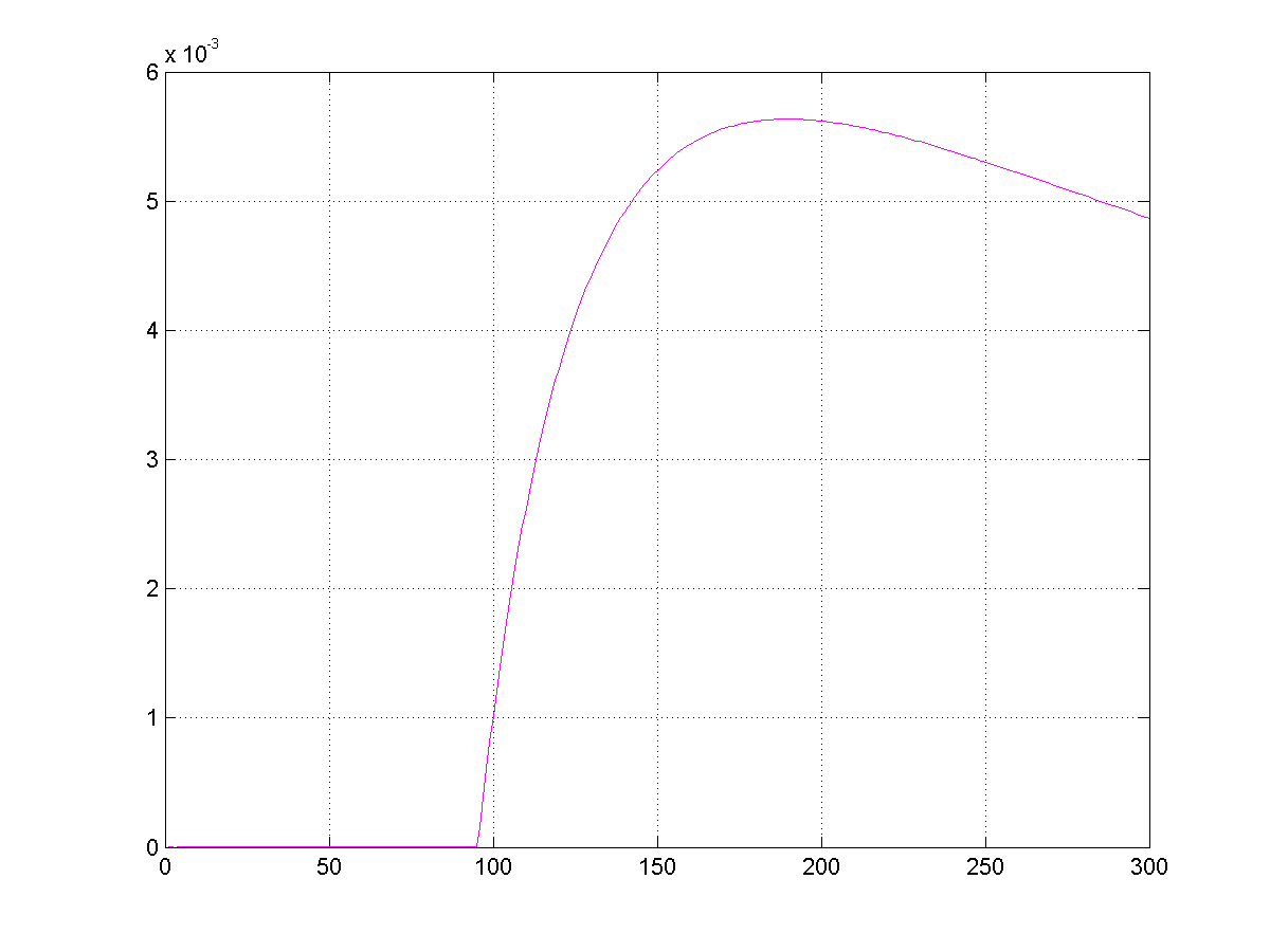
Fig. 11.4 Distribution of investments among the assets in the optimal solution of.

Please note that with our set-up there is exactly one asset with guaranteed return greater than $1$ – asset # 1 (bank savings, return 1.04, zero volatility). Consequently, the interval robust counterpart (11.38) prescribes to put our ` #1 in the bank, thus getting a 4% profit. In contrast to this, the diversified portfolio given by the optimal solution of (11.39) never yields profit less than 57.2%, and yields at average a 69.67% profit with pretty low (0.03) standard deviation. We see that in favorable circumstances the ellipsoidal robust counterpart of an uncertain linear program indeed is less conservative than, although basically as reliable as, the interval robust counterpart.

Finally, let us compare our results with those given by the nominal optimal solution. The latter prescribes to invest everything we have in the most promising asset (in our example this is the asset # 300 with a nominal return of 2.00 and volatility of 1.152). Assuming that the actual return is uniformly distributed in the corresponding interval and running 10,000 simulations, we get the following results:

Nominal optimal value: 2.0000
Actual returns over 10000 simulations:
Min=0.8483 Mean=1.9918 Max=3.1519 StD= 0.66

We see that the nominal solution results in a portfolio which is much more risky, although better at average, than the portfolio given by the robust solution.

11.3.4.2 Combined Interval-Ellipsoidal Robust Counterpart

We have considered the case when the coefficients $a_j$ of uncertain linear constraint (11.35) are affected by uncorrelated random perturbations symmetrically distributed in given intervals $[-{\sigma }_j,{\sigma }_j]$, and we have discussed two ways to model the uncertainty:

• The interval uncertainty model (the uncertainty set $\mathcal{U}$ is the box $B$), where we ignore the stochastic nature of the perturbations and their independence. This model yields the Interval Robust Counterpart (11.36);

• The ellipsoidal uncertainty model ($\mathcal{U}$ is the ellipsoid $E(\mathrm{\Omega })$), which takes into account the stochastic nature of data perturbations and yields the Ellipsoidal Robust Counterpart (11.37).

Please note that although for large $n$ the ellipsoid $E(\mathrm{\Omega })$ in its diameter, volume and average linear sizes is incomparably smaller than the box $B$, in the case of $\mathrm{\Omega }>1$ the ellipsoid $E(\mathrm{\Omega })$ in certain directions goes beyond the box. E.g. the ellipsoid $E(6)$, although much more narrow than $B$ in most of the directions, is 6 times wider than $B$ in the directions of the coordinate axes. Intuition says that it hardly makes sense to keep in the uncertainty set realizations of the data which are outside of $B$ and thus forbidden by our model of perturbations, so in the situation under consideration the intersection of $E(\mathrm{\Omega })$ and $B$ is a better model of the uncertainty set than the ellipsoid $E(\mathrm{\Omega })$ itself. What happens when the model of the uncertainty set is the combined interval-ellipsoidal uncertainty $\mathcal{U}(\mathrm{\Omega })=E(\mathrm{\Omega })\cap B$?

First, it turns out that the RC of (11.35) corresponding to the uncertainty set $\mathcal{U}(\mathrm{\Omega })$ is still given by a system of linear and conic quadratic inequalities, specifically the system

(11.40)$$\begin{array}{r}\begin{array}{rcccl}l& \le & \sum _{j=1}^n{a}_j^{\text{n}}{x}_j-\sum _{j=1}^n{\sigma }_j{y}_j-\mathrm{\Omega }\sqrt{\sum _{j=1}^n{\sigma }_j^2{u}_j^2},& & \\ & & \sum _{j=1}^n{a}_j^{\text{n}}{x}_j+\sum _{j=1}^n{\sigma }_j{z}_j+\mathrm{\Omega }\sqrt{\sum _{j=1}^n{\sigma }_j^2{v}_j^2}& \le & u,\\ -y_j& \le & x_j-u_j& \le & y_j,j=1,\dots ,n,\\ -z_j& \le & x_j-v_j& \le & z_j,j=1,\dots ,n.\end{array}\end{array}$$

Second, it turns out that our intuition is correct: As a model of uncertainty, $U(\mathrm{\Omega })$ is as reliable as the ellipsoid $E(\mathrm{\Omega })$. Specifically, if $x$ can be extended to a feasible solution of (11.40), then the probability for $x$ to satisfy a realization of (11.35) is $\ge 1-\exp \{-{\mathrm{\Omega }}^2/2\}$.

The conclusion is that if we have reasons to assume that the perturbations of uncertain coefficients in a constraint of an uncertain linear optimization problem are (a) random, (b) independent of each other, and (c) symmetrically distributed in given intervals, then it makes sense to associate with this constraint an interval-ellipsoidal model of uncertainty and use a system of linear and conic quadratic inequalities (11.40). Please note that when building the robust counterpart of an uncertain linear optimization problem, one can use different models of the uncertainty (e.g., interval, ellipsoidal, combined interval-ellipsoidal) for different uncertain constraints within the same problem.

Footnotes

[1]

NETLIB is a collection of LP’s, mainly of the real world origin, which is a standard benchmark for evaluating LP algorithms

[2]

Recall that in our discussion we have assumed the returns on different assets to be independent of each other. In reality, this is not so and this is why diversification of investments, although reducing the risk, never eliminates it completely

[3]

For the sake of simplicity, we assume that the bounds $l_c,u_c,l_x,u_x$ are not affected by uncertainty; extensions to the case when it is not so are evident.