3 Conic quadratic optimization

This chapter extends the notion of linear optimization with quadratic cones. Conic quadratic optimization, also known as second-order cone optimization, is a straightforward generalization of linear optimization, in the sense that we optimize a linear function under linear (in)equalities with some variables belonging to one or more (rotated) quadratic cones. We discuss the basic concept of quadratic cones, and demonstrate the surprisingly large flexibility of conic quadratic modeling.

3.1 Cones

Since this is the first place where we introduce a non-linear cone, it seems suitable to make our most important definition:

A set \(K\subseteq\real^n\) is called a convex cone if

• for every \(x,y\in K\) we have \(x+y\in K\),

• for every \(x\in K\) and \(\alpha\geq 0\) we have \(\alpha x\in K\).

For example a linear subspace of \(\real^n\), the positive orthant \(\real_{\geq 0}^n\) or any ray (half-line) starting at the origin are examples of convex cones. We leave it for the reader to check that the intersection of convex cones is a convex cone; this property enables us to assemble complicated optimization models from individual conic bricks.

3.1.1 Quadratic cones

We define the \(n\)-dimensional quadratic cone as

(3.1)\[\Q^n = \left \{ x\in \R^n \mid x_1 \geq \sqrt{x_2^2 + x_3^2 + \cdots + x_n^2} \right \}.\]

The geometric interpretation of a quadratic (or second-order) cone is shown in Fig. 3.1 for a cone with three variables, and illustrates how the boundary of the cone resembles an ice-cream cone. The 1-dimensional quadratic cone simply states nonnegativity \(x_1\geq 0\).

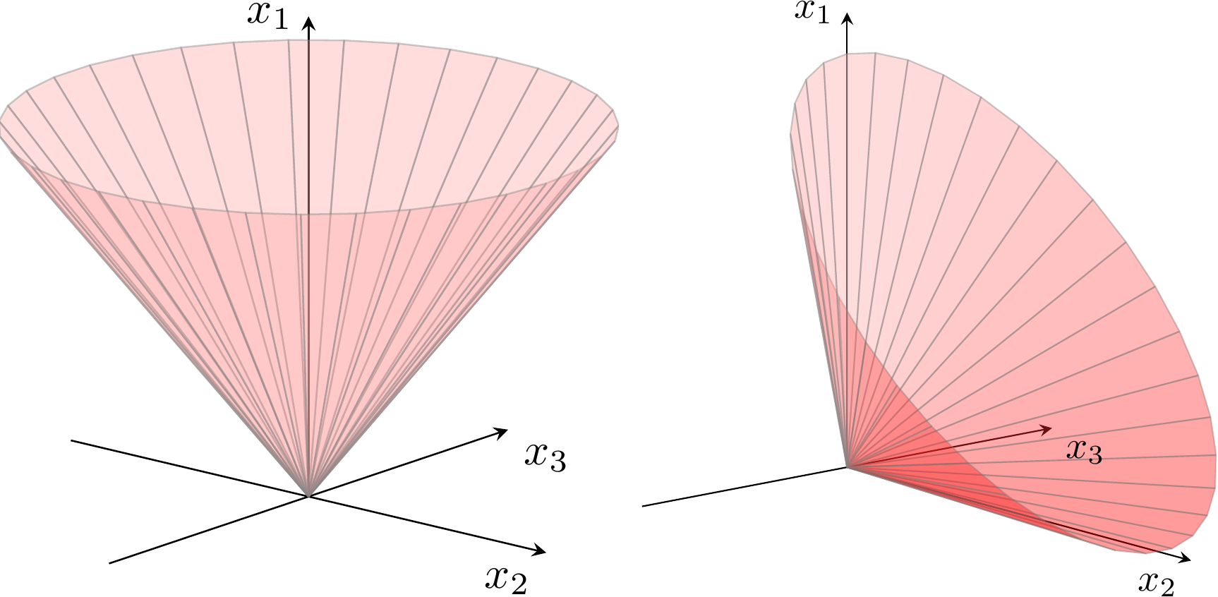
Fig. 3.1 Boundary of quadratic cone \(x_1\geq \sqrt{x_2^2+x_3^2}\) and rotated quadratic cone \(2x_1x_2\geq x_3^2\), \(x_1,x_2\geq 0\).

3.1.2 Rotated quadratic cones

An \(n-\)dimensional rotated quadratic cone is defined as

(3.2)\[\Q_r^n = \left \{ x\in \R^n \mid 2x_1 x_2 \geq x_3^2 + \cdots + x_n^2, \: x_1, x_2 \geq 0 \right \}.\]

As the name indicates, there is a simple relationship between quadratic and rotated quadratic cones. Define an orthogonal transformation

(3.3)\[\begin{split}T_n := \left[ \begin{array}{ccc} 1/\sqrt{2} & \hphantom{-}1/\sqrt{2} & \hphantom{-}0 \\ 1/\sqrt{2} & -1/\sqrt{2} & \hphantom{-}0 \\ 0 & \hphantom{-}0 & I_{n-2} \end{array} \right].\end{split}\]

Then it is easy to verify that

\[x \in \Q^n \quad \Longleftrightarrow \quad T_n x \in \Q^n_r,\]

and since \(T\) is orthogonal we call \(\Q_r^n\) a rotated cone; the transformation corresponds to a rotation of \(\pi/4\) in the \((x_1,x_2)\) plane. For example if \(x\in \Q^3\) and

\[\begin{split}\left[ \begin{array}{c}z_1 \\ z_2 \\ z_3 \end{array} \right] = \left[ \begin{array}{ccc} \frac{1}{\sqrt{2}} & \hphantom{-}\frac{1}{\sqrt{2}} & \hphantom{-}0 \\ \frac{1}{\sqrt{2}} & -\frac{1}{\sqrt{2}} & \hphantom{-}0 \\ 0 & \hphantom{-}0 & 1 \end{array} \right] \cdot \left[ \begin{array}{c}x_1 \\ x_2 \\ x_3 \end{array} \right] = \left[ \begin{array}{c}\frac{1}{\sqrt{2}}(x_1 + x_2)\\\frac{1}{\sqrt{2}}(x_1 - x_2)\\x_3 \end{array} \right]\end{split}\]

then

\[2 z_1 z_2 \geq z_3^2, \: z_1,z_2 \geq 0 \quad \Longrightarrow \quad (x_1^2 - x_2^2) \geq x_3^2, \: x_1 \geq 0,\]

and similarly we see that

\[x_1^2 \geq x_2^2 + x_3^2, \: x_1\geq 0 \quad \Longrightarrow \quad 2 z_1 z_2 \geq z_3^2, \: z_1, z_2 \geq 0.\]

Thus, one could argue that we only need quadratic cones \(\Q^n\), but there are many examples where using an explicit rotated quadratic cone \(\Q^n_r\) is more natural, as we will see next.

3.2 Conic quadratic modeling

In the following we describe several convex sets that can be modeled using conic quadratic formulations or, as we call them, are conic quadratic representable.

3.2.1 Absolute values

In Sec. 2.2.2 (Absolute value) we saw how to model \(|x|\leq t\) using two linear inequalities, but in fact the epigraph of the absolute value is just the definition of a two-dimensional quadratic cone, i.e.,

\[|x|\leq t \quad \Longleftrightarrow \quad (t, x) \in \Q^2.\]

3.2.2 Euclidean norms

The Euclidean norm of \(x\in \R^n\),

\[\| x \|_2 = \sqrt { x_1^2 + x_2^2 + \cdots + x_n^2 }\]

essentially defines the quadratic cone, i.e.,

\[\| x \|_2 \leq t \quad \Longleftrightarrow \quad (t, x)\in \Q^{n+1}.\]

The epigraph of the squared Euclidean norm can be described as the intersection of a rotated quadratic cone with an affine hyperplane,

\[x_1^2+\cdots+x_n^2 = \| x \|_2^2 \leq t \quad \Longleftrightarrow \quad (1/2, t, x)\in \Q_r^{n+2}.\]

3.2.3 Convex quadratic sets

Assume \(Q \in \R^{n \times n}\) is a symmetric positive semidefinite matrix. The convex inequality

\[(1/2)x^T Q x + c^T x + r \leq 0\]

may be rewritten as

(3.4)\[\begin{split} \begin{array}{rcl} t + c^T x + r & = & 0, \\ x^T Q x & \leq & 2 t. \\ \end{array}\end{split}\]

Since \(Q\) is symmetric positive semidefinite the epigraph

(3.5)\[x^T Q x \leq 2 t\]

is a convex set and there exists a matrix \(F\in \R^{k\times n}\) such that

(3.6)\[Q = F^T F\]

(see Sec. 6 (Semidefinite optimization) for properties of semidefinite matrices). For instance \(F\) could be the Cholesky factorization of \(Q\). Then

\[x^TQx = x^TF^TFx=\|Fx\|_2^2\]

and we have an equivalent characterization of (3.5) as

\[(1/2)x^T Q x \leq t \quad \iff \quad (t,1,F x) \in \Q_r^{2+k}.\]

Frequently \(Q\) has the structure

\[Q = I + F^T F\]

where \(I\) is the identity matrix, so

\[x^T Q x = x^T x + x^T F^T F x = \|x\|_2^2+\|Fx\|_2^2\]

and hence

\[\begin{split}\left(t,1,\left[\begin{array}{c}I\\ F\end{array}\right]x \right) \in \Q_r^{2+n+k}\end{split}\]

is a conic quadratic representation of (3.5) in this case.

3.2.4 Second-order cones

A second-order cone is occasionally specified as

(3.7)\[\| Ax + b \|_2 \leq c^T x + d\]

where \(A \in \R^{m\times n}\) and \(c \in \R^n\). The formulation (3.7) is simply

(3.8)\[(c^T x + d, Ax + b) \in \Q^{m+1}\]

or equivalently

(3.9)\[\begin{split}\begin{array}{rcl} s & = & A x + b, \\ t & = & c^T x + d, \\ (t,s) & \in & \Q^{m+1}. \end{array}\end{split}\]

As will be explained in Sec. 8 (Duality in conic optimization), we refer to (3.8) as the dual form and (3.9) as the primal form. An alternative characterization of (3.7) is

(3.10)\[\|Ax + b\|^2_2 - (c^T x + d)^2 \leq 0, \qquad c^T x+ d \geq 0\]

which shows that certain quadratic inequalities are conic quadratic representable.

3.2.5 Simple sets involving power functions

Some power-like inequalities are conic quadratic representable, even though it need not be obvious at first glance. For example, we have

\[|t| \leq \sqrt{x}, \, x \geq 0 \iff (x,1/2,t) \in \Q_r^3,\]

or in a similar fashion

\[t \geq \frac{1}{x}, \, x \geq 0 \iff (x,t,\sqrt{2}) \in \Q_r^3.\]

For a more complicated example, consider the constraint

\[t \geq x^{3/2}, x\geq 0.\]

This is equivalent to a statement involving two cones and an extra variable

\[(s,t,x), (x,1/8,s) \in \Q_r^3\]

because

\[2st\geq x^2,\ 2\cdot\frac{1}{8}x\geq s^2, \implies 4s^2t^2\cdot\frac{1}{4}x\geq x^4\cdot s^2 \implies t\geq x^{3/2}.\]

In practice power-like inequalities representable with similar tricks can often be expressed much more naturally using the power cone (see Sec. 4 (The power cones)), so we will not dwell on these examples much longer.

3.2.6 Rational functions

A general non-degenerate rational function of one variable \(f(x)=\frac{ax+b}{gx+h}\) can always be written in the form \(f(x)=p+\frac{q}{gx+h}\), and when \(q>0\) it is convex on the set where \(gx+h>0\). The conic quadratic model of

\[t \geq p+\frac{q}{gx+h}, \quad gx+h>0, \quad q>0\]

with variables \(t,x\) can be written as:

\[(t-p, gx+h, \sqrt{2q}) \in \Q_r^3.\]

We can generalize it to a quadratic-over-linear function \(f(x)=\frac{ax^2+bx+c}{gx+h}\). By performing long polynomial division we can write it as \(f(x)=rx+s+\frac{q}{gx+h}\), and as before it is convex when \(q>0\) on the set where \(gx+h>0\). In particular

\[t \geq rx+s+\frac{q}{gx+h}, \quad gx+h>0, \quad q>0\]

can be written as

\[(t-rx-s, gx+h, \sqrt{2q}) \in \Q_r^3.\]

In both cases the argument boils down to the observation that the target function is a sum of an affine expression and the inverse of a positive affine expression, see Sec. 3.2.5 (Simple sets involving power functions).

3.2.7 Harmonic mean

Consider next the hypograph of the harmonic mean,

\[\left (\frac{1}{n} \sum_{i=1}^n x_i^{-1} \right )^{-1} \geq t\geq 0, \quad x\geq 0.\]

It is not obvious that the inequality defines a convex set, nor that it is conic quadratic representable. However, we can rewrite it in the form

\[\sum_{i=1}^n \frac{t^2}{x_i} \leq nt,\]

which suggests the conic representation:

(3.11)\[ 2 x_i z_i \geq t^2, \quad x_i, z_i\geq 0, \quad 2\sum_{i=1}^n z_i = nt.\]

Alternatively, in case \(n=2\), the hypograph of the harmonic mean can be represented by a single quadratic cone:

(3.12)\[\left( x_1 + x_2 - t/2, x_1, x_2, t/2 \right) \in \Q^{4}.\]

As this representation generalizes the harmonic mean to all points \(x_1 + x_2 \geq 0\), as implied by (3.12), the variable bounds \(x\geq 0\) and \(t\geq 0\) have to be added seperately if so desired.

3.2.8 Quadratic forms with one negative eigenvalue

Assume that \(A \in \R^{n \times n}\) is a symmetric matrix with exactly one negative eigenvalue, i.e., \(A\) has a spectral factorization (i.e., eigenvalue decomposition)

\[A = Q \Lambda Q^T = -\alpha_1 q_1 q_1^T + \sum_{i=2}^n \alpha_i q_i q_i^T,\]

where \(Q^T Q = I\), \(\Lambda=\Diag(-\alpha_1, \alpha_2, \dots, \alpha_n)\), \(\alpha_i \geq 0\). Then

\[x^T A x \leq 0\]

is equivalent to

(3.13)\[\sum_{j=2}^n \alpha_j (q_j^T x)^2 \leq \alpha_1 (q_1^T x)^2.\]

This shows \(x^T A x \leq 0\) to be a union of two convex subsets, each representable by a quadratic cone. For example, assuming \(q_1^T x \geq 0\), we can characterize (3.13) as

(3.14)\[(\sqrt{\alpha_1}q_1^Tx, \sqrt{\alpha_2}q_2^Tx, \dots, \sqrt{\alpha_n}q_n^Tx ) \in \Q^{n}.\]

3.2.9 Ellipsoidal sets

The set

\[{\cal E} = \{ x\in \R^n \mid \| P(x-c) \|_2 \leq 1 \}\]

describes an ellipsoid centred at \(c\). It has a natural conic quadratic representation, i.e., \(x\in {\cal E}\) if and only if

\[x\in{\cal E} \iff (1, P(x-c)) \in \Q^{n+1}.\]

3.3 Conic quadratic case studies

3.3.1 Quadratically constrained quadratic optimization

A general convex quadratically constrained quadratic optimization problem can be written as

(3.15)\[\begin{split}\begin{array}{ll} \mbox{minimize} & (1/2)x^T Q_0 x + c_0^T x + r_0\\ \mbox{subject to}& (1/2)x^T Q_i x + c_i^T x + r_i \leq 0, \quad i=1,\dots,p, \end{array}\end{split}\]

where all \(Q_i\in\real^{n\times n}\) are symmetric positive semidefinite. Let

\[Q_i = F_i^T F_i, \quad i=0,\dots,p,\]

where \(F_i \in \R^{k_i \times n}\). Using the formulations in Sec. 3.2.3 (Convex quadratic sets) we then get an equivalent conic quadratic problem

(3.16)\[\begin{split}\begin{array}{lll} \mbox{minimize} & t_0 + c_0^T x + r_0 & \\ \mbox{subject to} & t_i + c_i^T x + r_i = 0, & i=1,\dots,p, \\ & (t_i,1,F_i x) \in \Q_r^{k_i+2},& i=0,\dots,p. \\ \end{array}\end{split}\]

Assume next that \(k_i\), the number of rows in \(F_i\), is small compared to \(n\). Storing \(Q_i\) requires about \(n^2/2\) space whereas storing \(F_i\) then only requires \(nk_i\) space. Moreover, the amount of work required to evaluate \(x^T Q_i x\) is proportional to \(n^2\) whereas the work required to evaluate \(x^T F_i^T F_ i x = \| F_i x \|^2\) is proportional to \(nk_i\) only. In other words, if \(Q_i\) have low rank, then (3.16) will require much less space and time to solve than (3.15). We will study the reformulation (3.16) in much more detail in Sec. 10 (Quadratic optimization).

3.3.2 Robust optimization with ellipsoidal uncertainties

Often in robust optimization some of the parameters in the model are assumed to be unknown exactly, but there is a simple set describing the uncertainty. For example, for a standard linear optimization problem we may wish to find a robust solution for all objective vectors \(c\) in an ellipsoid

\[{\cal E} = \{ c\in \R^n \mid c = Fy + g, \: \| y \|_2 \leq 1 \}.\]

A common approach is then to optimize for the worst-case scenario for \(c\), so we get a robust version

(3.17)\[\begin{split}\begin{array}{ll} \mbox{minimize}& \sup_{c\in {\cal E}} c^T x\\ \mbox{subject to}& Ax = b,\\ & x\geq 0. \end{array}\end{split}\]

The worst-case objective can be evaluated as

\[\sup_{c\in {\cal E}} c^T x = g^T x + \sup_{\| y \|_2 \leq 1} y^T F^T x = g^T x + \| F^T x\|_2\]

where we used that \(\sup_{\| u \|_2\leq 1} v^T u = (v^T v)/\|v\|_2=\|v\|_2\). Thus the robust problem (3.17) is equivalent to

\[\begin{split}\begin{array}{ll} \mbox{minimize}& g^T x + \|F^T x \|_2\\ \mbox{subject to}& Ax = b,\\ & x\geq 0, \end{array}\end{split}\]

which can be posed as a conic quadratic problem

(3.18)\[\begin{split}\begin{array}{ll} \mbox{minimize}& g^T x + t\\ \mbox{subject to}& Ax = b,\\ & (t,F^T x) \in \Q^{n+1},\\ & x \geq 0. \end{array}\end{split}\]

3.3.3 Markowitz portfolio optimization

In classical Markowitz portfolio optimization we consider investment in \(n\) stocks or assets held over a period of time. Let \(x_i\) denote the amount we invest in asset \(i\), and assume a stochastic model where the return of the assets is a random variable \(r\) with known mean

\[\mu = \mathbf{E}r\]

and covariance

\[\Sigma = \mathbf{E}(r-\mu)(r-\mu)^T.\]

The return of our investment is also a random variable \(y = r^Tx\) with mean (or expected return)

\[\mathbf{E}y = \mu^T x\]

and variance (or risk)

\[(y - \mathbf{E}y)^2 = x^T \Sigma x.\]

We then wish to rebalance our portfolio to achieve a compromise between risk and expected return, e.g., we can maximize the expected return given an upper bound \(\gamma\) on the tolerable risk and a constraint that our total investment is fixed,

(3.19)\[\begin{split}\begin{array}{ll} \mbox{maximize}& \mu^T x\\ \mbox{subject to}& x^T \Sigma x \leq \gamma\\ & e^T x = 1\\ & x \geq 0. \end{array}\end{split}\]

Suppose we factor \(\Sigma = GG^T\) (e.g., using a Cholesky or a eigenvalue decomposition). We then get a conic formulation

(3.20)\[\begin{split}\begin{array}{ll} \mbox{maximize}& \mu^T x\\ \mbox{subject to}& (\sqrt{\gamma}, G^Tx) \in \Q^{n+1}\\ & e^T x = 1\\ & x \geq 0. \end{array}\end{split}\]

In practice both the average return and covariance are estimated using historical data. A recent trend is then to formulate a robust version of the portfolio optimization problem to combat the inherent uncertainty in those estimates, e.g., we can constrain \(\mu\) to an ellipsoidal uncertainty set as in Sec. 3.3.2 (Robust optimization with ellipsoidal uncertainties).

It is also common that the data for a portfolio optimization problem is already given in the form of a factor model \(\Sigma=F^TF\) of \(\Sigma=I+F^TF\) and a conic quadratic formulation as in Sec. 3.3.1 (Quadratically constrained quadratic optimization) is most natural. For more details see Sec. 10.3 (Example: Factor model).

3.3.4 Maximizing the Sharpe ratio

Continuing the previous example, the Sharpe ratio defines an efficiency metric of a portfolio as the expected return per unit risk, i.e.,

\[S(x) = \frac {\mu^T x - r_f}{ (x^T \Sigma x)^{1/2}},\]

where \(r_f\) denotes the return of a risk-free asset. We assume that there is a portfolio with \(\mu^T x>r_f\), so maximizing the Sharpe ratio is equivalent to minimizing \(1/S(x)\). In other words, we have the following problem

\[\begin{split}\begin{array}{lccc} \text{minimize} & \frac{\| G^T x \|}{\mu^T x - r_f}\\ \text{subject to} & e^Tx & = & 1,\\ & x &\geq & 0. \end{array}\end{split}\]

The objective has the same nature as a quotient of two affine functions we studied in Sec. 2.2.5 (Homogenization). We reformulate the problem in a similar way, introducing a scalar variable \(z\geq 0\) and a variable transformation

\[y = z x.\]

Since a positive \(z\) can be chosen arbitrarily and \((\mu - r_fe)^T x>0\), we can without loss of generality assume that

\[(\mu -r_fe)^T y = 1.\]

Thus, we obtain the following conic problem for maximizing the Sharpe ratio,

\[\begin{split}\begin{array}{lccc} \text{minimize} & t\\ \text{subject to} & (t, G^Ty) & \in &\Q^{k+1},\\ & e^Ty & = & z, \\ & (\mu -r_fe)^T y& = & 1,\\ & y,z & \geq & 0, \end{array}\end{split}\]

and we recover \(x = y/z\).

3.3.5 A resource constrained production and inventory problem

The resource constrained production and inventory problem [Zie82] can be formulated as follows:

(3.21)\[\begin{split}\begin{array}{lll} \mbox{minimize} & \sum_{j=1}^n (d_j x_j + e_j/x_j) & \\ \mbox{subject to} & \sum_{j=1}^n r_j x_j \leq b, &\\ & x_j \geq 0, & j=1,\dots,n, \end{array}\end{split}\]

where \(n\) denotes the number of items to be produced, \(b\) denotes the amount of common resource, and \(r_j\) is the consumption of the limited resource to produce one unit of item \(j\). The objective function represents inventory and ordering costs. Let \(c_j^p\) denote the holding cost per unit of product \(j\) and \(c_j^r\) denote the rate of holding costs, respectively. Further, let

\[d_j = \frac{c_j^p c_j^r}{2}\]

so that

\[d_j x_j\]

is the average holding costs for product \(j\). If \(D_j\) denotes the total demand for product \(j\) and \(c_j^o\) the ordering cost per order of product \(j\) then let

\[e_j = c_j^o D_j\]

and hence

\[\frac{e_j}{x_j} = \frac{c_j^o D_j}{x_j}\]

is the average ordering costs for product \(j\). In summary, the problem finds the optimal batch size such that the inventory and ordering cost are minimized while satisfying the constraints on the common resource. Given \(d_j, e_j \geq 0\) problem (3.21) is equivalent to the conic quadratic problem

\[\begin{split}\begin{array}{lll} \mbox{minimize} & \sum_{j=1}^n (d_j x_j + e_j t_j) \\ \mbox{subject to} & \sum_{j=1}^n r_j x_j \leq b,\\ & (t_j, x_j, \sqrt{2}) \in \Q_r^3, & j=1,\dots,n. \end{array}\end{split}\]

It is not always possible to produce a fractional number of items. In such case \(x_j\) should be constrained to be integers. See Sec. 9 (Mixed integer optimization).