11.1 Portfolio Optimization

In this section the Markowitz portfolio optimization problem and variants are implemented using Fusion API for Python.

• Basic Markowitz model

• Efficient frontier

• Factor model and efficiency

• Market impact costs

• Transaction costs

• Cardinality constraints

11.1.1 The Basic Model

The classical Markowitz portfolio optimization problem considers investing in $n$ stocks or assets held over a period of time. Let $x_j$ denote the amount invested in asset $j$, and assume a stochastic model where the return of the assets is a random variable $r$ with known mean

$$\mu =\mathbf{E}r$$

and covariance

$$\mathrm{\Sigma }=\mathbf{E}(r-\mu )(r-\mu {)}^T.$$

The return of the investment is also a random variable $y=r^{T}x$ with mean (or expected return)

$$\mathbf{E}y={\mu }^{T}x$$

and variance

$$\mathbf{E}(y-\mathbf{E}y{)}^2=x^T\mathrm{\Sigma }x.$$

The standard deviation

$$\sqrt{x^T\mathrm{\Sigma }x}$$

is usually associated with risk.

The problem facing the investor is to rebalance the portfolio to achieve a good compromise between risk and expected return, e.g., maximize the expected return subject to a budget constraint and an upper bound (denoted $\gamma$) on the tolerable risk. This leads to the optimization problem

(11.1)$$\begin{array}{r}\begin{array}{lrcl}\text{maximize}& {\mu }^{T}x& & \\ \text{subject to}& e^{T}x& =& w+e^T{x}^0,\\ & x^T\mathrm{\Sigma }x& \le & {\gamma }^2,\\ & x& \ge & 0.\end{array}\end{array}$$

The variables $x$ denote the investment i.e. $x_j$ is the amount invested in asset $j$ and $x_j^0$ is the initial holding of asset $j$. Finally, $w$ is the initial amount of cash available.

A popular choice is $x^0=0$ and $w=1$ because then $x_j$ may be interpreted as the relative amount of the total portfolio that is invested in asset $j$.

Since $e$ is the vector of all ones then

$$e^{T}x=\sum _{j=1}^n{x}_j$$

is the total investment. Clearly, the total amount invested must be equal to the initial wealth, which is

$$w+e^T{x}^0.$$

This leads to the first constraint

$$e^{T}x=w+e^T{x}^0.$$

The second constraint

$$x^T\mathrm{\Sigma }x\le {\gamma }^2$$

ensures that the variance, is bounded by the parameter ${\gamma }^2$. Therefore, $\gamma$ specifies an upper bound of the standard deviation (risk) the investor is willing to undertake. Finally, the constraint

$$x_j\ge 0$$

excludes the possibility of short-selling. This constraint can of course be excluded if short-selling is allowed.

The covariance matrix $\mathrm{\Sigma }$ is positive semidefinite by definition and therefore there exist a matrix $G\in {\mathbb{R}}^{n\times k}$ such that

(11.2)$$\mathrm{\Sigma }=G{G}^T.$$

In general the choice of $G$ is not unique and one possible choice of $G$ is the Cholesky factorization of $\mathrm{\Sigma }$. However, in many cases another choice is better for efficiency reasons as discussed in Sec. 11.1.3 (Factor model and efficiency). For a given $G$ we have that

$$\begin{array}{r}\begin{array}{lll}{x}^T\mathrm{\Sigma }x& =& x^{T}G{G}^{T}x\\ & =& {\Vert G^{T}x\Vert }^2.\end{array}\end{array}$$

Hence, we may write the risk constraint as

$$\gamma \ge \Vert G^{T}x\Vert$$

or equivalently

$$(\gamma ,G^{T}x)\in {\mathcal{Q}}^{k+1},$$

where ${\mathcal{Q}}^{k+1}$ is the $(k+1)$-dimensional quadratic cone. Note that specifically when $G$ is derived using Cholesky factorization, $k=n$.

Therefore, problem (11.1) can be written as

(11.3)$$\begin{array}{r}\begin{array}{lrcl}\text{maximize}& {\mu }^{T}x& & \\ \text{subject to}& e^{T}x& =& w+e^T{x}^0,\\ & (\gamma ,G^{T}x)& \in & {\mathcal{Q}}^{k+1},\\ & x& \ge & 0,\end{array}\end{array}$$

which is a conic quadratic optimization problem that can easily be formulated and solved with Fusion API for Python. Subsequently we will use the example data

$$\mu ={\left[\begin{array}{c}0.0720,0.1552,0.1754,0.0898,0.4290,0.3929,0.3217,0.1838\end{array}\right]}^T$$

and

$$\begin{array}{r}\mathrm{\Sigma }=\left[\begin{array}{cccccccc}0.0946& 0.0374& 0.0349& 0.0348& 0.0542& 0.0368& 0.0321& 0.0327\\ 0.0374& 0.0775& 0.0387& 0.0367& 0.0382& 0.0363& 0.0356& 0.0342\\ 0.0349& 0.0387& 0.0624& 0.0336& 0.0395& 0.0369& 0.0338& 0.0243\\ 0.0348& 0.0367& 0.0336& 0.0682& 0.0402& 0.0335& 0.0436& 0.0371\\ 0.0542& 0.0382& 0.0395& 0.0402& 0.1724& 0.0789& 0.0700& 0.0501\\ 0.0368& 0.0363& 0.0369& 0.0335& 0.0789& 0.0909& 0.0536& 0.0449\\ 0.0321& 0.0356& 0.0338& 0.0436& 0.0700& 0.0536& 0.0965& 0.0442\\ 0.0327& 0.0342& 0.0243& 0.0371& 0.0501& 0.0449& 0.0442& 0.0816\end{array}\right].\end{array}$$

Using Cholesky factorization, this implies

$$\begin{array}{r}{G}^T=\left[\begin{array}{cccccccc}0.3076& 0.1215& 0.1134& 0.1133& 0.1763& 0.1197& 0.1044& 0.1064\\ 0.& 0.2504& 0.0995& 0.0916& 0.0669& 0.0871& 0.0917& 0.0851\\ 0.& 0.& 0.1991& 0.0587& 0.0645& 0.0737& 0.0647& 0.0191\\ 0.& 0.& 0.& 0.2088& 0.0493& 0.0365& 0.0938& 0.0774\\ 0.& 0.& 0.& 0.& 0.3609& 0.1257& 0.1016& 0.0571\\ 0.& 0.& 0.& 0.& 0.& 0.2155& 0.0566& 0.0619\\ 0.& 0.& 0.& 0.& 0.& 0.& 0.2251& 0.0333\\ 0.& 0.& 0.& 0.& 0.& 0.& 0.& 0.2202\end{array}\right]\end{array}$$

In Sec. 11.1.3 (Factor model and efficiency), we present a different way of obtaining $G$ based on a factor model, that leads to more efficient computation.

Why a Conic Formulation?

Problem (11.1) is a convex quadratically constrained optimization problem that can be solved directly using MOSEK. Why then reformulate it as a conic quadratic optimization problem (11.3)? The main reason for choosing a conic model is that it is more robust and usually solves faster and more reliably. For instance it is not always easy to numerically validate that the matrix $\mathrm{\Sigma }$ in (11.1) is positive semidefinite due to the presence of rounding errors. It is also very easy to make a mistake so $\mathrm{\Sigma }$ becomes indefinite. These problems are completely eliminated in the conic formulation.

Moreover, observe the constraint

$$\Vert G^{T}x\Vert \le \gamma$$

more numerically robust than

$$x^T\mathrm{\Sigma }x\le {\gamma }^2$$

for very small and very large values of $\gamma$. Indeed, if say $\gamma \approx {10}^4$ then ${\gamma }^2\approx {10}^8$, which introduces a scaling issue in the model. Hence, using conic formulation we work with the standard deviation instead of variance, which usually gives rise to a better scaled model.

Example code

Listing 11.1 demonstrates how the basic Markowitz model (11.3) is implemented.

Listing 11.1 Code implementing problem (11.3). Click here to download.

def BasicMarkowitz(n,mu,GT,x0,w,gamma):
    
    with  Model("Basic Markowitz") as M:

        # Redirect log output from the solver to stdout for debugging. 
        # if uncommented.
        # M.setLogHandler(sys.stdout) 
        
        # Defines the variables (holdings). Shortselling is not allowed.
        x = M.variable("x", n, Domain.greaterThan(0.0))
        
        #  Maximize expected return
        M.objective('obj', ObjectiveSense.Maximize, x.T @ mu)
        
        # The amount invested  must be identical to initial wealth
        M.constraint('budget', Expr.sum(x) == w+sum(x0))
        
        # Imposes a bound on the risk
        M.constraint('risk', Expr.vstack(gamma, GT @ x) == Domain.inQCone())
        #M.constraint('risk', Expr.vstack(gamma, 0.5, Expr.mul(GT, x)), Domain.inRotatedQCone())

        # Solves the model.
        M.solve()

        # Check if the solution is an optimal point
        solsta = M.getPrimalSolutionStatus()
        if (solsta != SolutionStatus.Optimal):
            # See https://docs.mosek.com/latest/pythonfusion/accessing-solution.html about handling solution statuses.
            raise Exception(f"Unexpected solution status: {solsta}")

        return np.dot(mu, x.level()), x.level()

The source code should be self-explanatory except perhaps for

        M.constraint('risk', Expr.vstack(gamma, GT @ x) == Domain.inQCone())
        #M.constraint('risk', Expr.vstack(gamma, 0.5, Expr.mul(GT, x)), Domain.inRotatedQCone())

where the linear expression

$$(\gamma ,G^{T}x)$$

is created using the Expr.vstack operator. Finally, the linear expression must lie in a quadratic cone implying

$$\gamma \ge \Vert G^{T}x\Vert .$$

11.1.2 The Efficient Frontier

The portfolio computed by the Markowitz model is efficient in the sense that there is no other portfolio giving a strictly higher return for the same amount of risk. An efficient portfolio is also sometimes called a Pareto optimal portfolio. Clearly, an investor should only invest in efficient portfolios and therefore it may be relevant to present the investor with all efficient portfolios so the investor can choose the portfolio that has the desired tradeoff between return and risk.

Given a nonnegative $\alpha$ the problem

(11.4)$$\begin{array}{r}\begin{array}{ll}\text{maximize}& {\mu }^{T}x-\alpha x^T\mathrm{\Sigma }x\\ \text{subject to}& e^{T}x=w+e^T{x}^0,\\ & x\ge 0.\end{array}\end{array}$$

is one standard way to trade the expected return against penalizing variance. Note that, in contrast to the previous example, we explicitly use the variance ($\Vert G^{T}x{\Vert }_2^2$) rather than standard deviation ($\Vert G^{T}x{\Vert }_2$), therefore the conic model includes a rotated quadratic cone:

(11.5)$$\begin{array}{r}\begin{array}{lrcll}\text{maximize}& {\mu }^{T}x-\alpha s& & & \\ \text{subject to}& e^{T}x& =& w+e^T{x}^0,& \\ & (s,0.5,G^{T}x)& \in & Q_r^{k+2}& (\text{equiv. to}s\ge \Vert G^{T}x{\Vert }_2^2=x^T\mathrm{\Sigma }x),\\ & x& \ge & 0.& \end{array}\end{array}$$

The parameter $\alpha$ specifies the tradeoff between expected return and variance. Ideally the problem (11.4) should be solved for all values $\alpha \ge 0$ but in practice it is impossible. Using the example data from Sec. 11.1.1 (The Basic Model), the optimal values of return and variance for several values of $\alpha$ are shown in the figure.

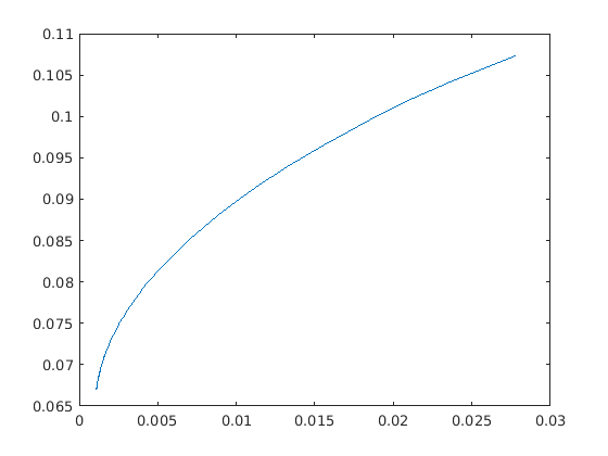
Fig. 11.1 The efficient frontier for the sample data.

Example code

Listing 11.2 demonstrates how to compute the efficient portfolios for several values of $\alpha$.

Listing 11.2 Code for the computation of the efficient frontier based on problem (11.4). Click here to download.

def EfficientFrontier(n,mu,GT,x0,w,alphas):

    with Model("Efficient frontier") as M:
        frontier = []

        # Defines the variables (holdings). Shortselling is not allowed.
        x = M.variable("x", n, Domain.greaterThan(0.0)) # Portfolio variables
        s = M.variable("s", 1, Domain.unbounded())      # Variance variable

        # Total budget constraint
        M.constraint('budget', Expr.sum(x) == w+sum(x0))

        # Computes the risk
        M.constraint('variance', Expr.vstack(s, 0.5, GT @ x), Domain.inRotatedQCone())

        # Define objective as a weighted combination of return and variance
        alpha = M.parameter()
        M.objective('obj', ObjectiveSense.Maximize, x.T @ mu - s * alpha)
        
        # Solve multiple instances by varying the parameter alpha
        for a in alphas:
            alpha.setValue(a)

            M.solve()

            # Check if the solution is an optimal point
            solsta = M.getPrimalSolutionStatus()
            if (solsta != SolutionStatus.Optimal):
                # See https://docs.mosek.com/latest/pythonfusion/accessing-solution.html about handling solution statuses.
                raise Exception(f"Unexpected solution status: {solsta}")

            frontier.append((a, np.dot(mu,x.level()), s.level()[0]))

        return frontier

Note that we defined $\alpha$ as a model parameter and used it to parametrize the objective. This way we were able to reuse the same model for all solves along the efficient frontier, simply changing the value of $\alpha$ between the solves.

11.1.3 Factor model and efficiency

In practice it is often important to solve the portfolio problem very quickly. Therefore, in this section we discuss how to improve computational efficiency at the modeling stage.

The computational cost is of course to some extent dependent on the number of constraints and variables in the optimization problem. However, in practice a more important factor is the sparsity: the number of nonzeros used to represent the problem. Indeed it is often better to focus on the number of nonzeros in $G$ see (11.2) and try to reduce that number by for instance changing the choice of $G$.

In other words if the computational efficiency should be improved then it is always good idea to start with focusing at the covariance matrix. As an example assume that

$$\mathrm{\Sigma }=D+V{V}^T$$

where $D$ is a positive definite diagonal matrix. Moreover, $V$ is a matrix with $n$ rows and $k$ columns. Such a model for the covariance matrix is called a factor model and usually $k$ is much smaller than $n$. In practice $k$ tends to be a small number independent of $n$, say less than 100.

One possible choice for $G$ is the Cholesky factorization of $\mathrm{\Sigma }$ which requires storage proportional to $n(n+1)/2$. However, another choice is

$$\begin{array}{r}G=\left[\begin{array}{cc}{D}^{1/2}& V\end{array}\right]\end{array}$$

because then

$$G{G}^T=D+V{V}^T.$$

This choice requires storage proportional to $n+kn$ which is much less than for the Cholesky choice of $G$. Indeed assuming $k$ is a constant storage requirements are reduced by a factor of $n$.

The example above exploits the so-called factor structure and demonstrates that an alternative choice of $G$ may lead to a significant reduction in the amount of storage used to represent the problem. This will in most cases also lead to a significant reduction in the solution time.

The lesson to be learned is that it is important to investigate how the covariance matrix is formed. Given this knowledge it might be possible to make a special choice for $G$ that helps reducing the storage requirements and enhance the computational efficiency. More details about this process can be found in [And13].

Factor model in finance

Factor model structure is typical in financial context. It is common to model security returns as the sum of two components using a factor model. The first component is the linear combination of a small number of factors common among a group of securities. The second component is a residual, specific to each security. It can be written as $R=\sum _j{\beta }_j{F}_j+\theta$, where $R$ is a random variable representing the return of a security at a particular point in time, $F_j$ is the random variable representing the common factor $j$, ${\beta }_j$ is the exposure of the return to factor $j$, and $\theta$ is the specific component.

Such a model will result in the covariance structure

$$\mathrm{\Sigma }={\mathrm{\Sigma }}_{\theta }+\beta {\mathrm{\Sigma }}_F{\beta }^T,$$

where ${\mathrm{\Sigma }}_F$ is the covariance of the factors and ${\mathrm{\Sigma }}_{\theta }$ is the residual covariance. This structure is of the form discussed earlier with $D={\mathrm{\Sigma }}_{\theta }$ and $V=\beta P$, assuming the decomposition ${\mathrm{\Sigma }}_F=P{P}^T$. If the number of factors $k$ is low and ${\mathrm{\Sigma }}_{\theta }$ is diagonal, we get a very sparse $G$ that provides the storage and solution time benefits.

Example code

Here we will work with the example data of a two-factor model ($k=2$) built using the variables

$$\begin{array}{r}\beta =\left[\begin{array}{cc}0.4256& 0.1869\\ 0.2413& 0.3877\\ 0.2235& 0.3697\\ 0.1503& 0.4612\\ 1.5325& -0.2633\\ 1.2741& -0.2613\\ 0.6939& 0.2372\\ 0.5425& 0.2116\end{array}\right],\end{array}$$

$$\theta =[0.0720,0.0508,0.0377,0.0394,0.0663,0.0224,0.0417,0.0459],$$

and the factor covariance matrix is

$$\begin{array}{r}{\mathrm{\Sigma }}_F=\left[\begin{array}{cc}0.0620& 0.0577\\ 0.0577& 0.0908\end{array}\right],\end{array}$$

giving

$$\begin{array}{r}P=\left[\begin{array}{cc}0.2491& 0.\\ 0.2316& 0.1928\end{array}\right].\end{array}$$

Then the matrix $G$ would look like

$$\begin{array}{r}G=\left[\begin{array}{cc}\beta P& {\mathrm{\Sigma }}_{\theta }^{1/2}\end{array}\right]=\left[\begin{array}{cccccccccc}0.1493& 0.0360& 0.2683& 0.& 0.& 0.& 0.& 0.& 0.& 0.\\ 0.1499& 0.0747& 0.& 0.2254& 0.& 0.& 0.& 0.& 0.& 0.\\ 0.1413& 0.0713& 0.& 0.& 0.1942& 0.& 0.& 0.& 0.& 0.\\ 0.1442& 0.0889& 0.& 0.& 0.& 0.1985& 0.& 0.& 0.& 0.\\ 0.3207& -0.0508& 0.& 0.& 0.& 0.& 0.2576& 0.& 0.& 0.\\ 0.2568& -0.0504& 0.& 0.& 0.& 0.& 0.& 0.1497& 0.& 0.\\ 0.2277& 0.0457& 0.& 0.& 0.& 0.& 0.& 0.& 0.2042& 0.\\ 0.1841& 0.0408& 0.& 0.& 0.& 0.& 0.& 0.& 0.& 0.2142\end{array}\right].\end{array}$$

This matrix is indeed very sparse.

In general, we get an $n\times (n+k)$ size matrix this way with $k$ full columns and an $n\times n$ diagonal part. In order to maintain a sparse representation we do not construct the matrix $G$ explicitly in the code but instead work with two pieces of data: the dense matrix $G_{\mathrm{factor}}=\beta P$ of shape $n\times k$ and the diagonal vector $\theta$ of length $n$.

Example code

In the following we demonstrate how to write code to compute the matrix $G_{\mathrm{factor}}$ of the factor model. We start with the inputs

Listing 11.3 Inputs for the computation of the matrix $G_{\mathrm{factor}}$ from the factor model.

    B = np.array([
        [0.4256, 0.1869],
        [0.2413, 0.3877],
        [0.2235, 0.3697],
        [0.1503, 0.4612],
        [1.5325, -0.2633],
        [1.2741, -0.2613],
        [0.6939, 0.2372],
        [0.5425, 0.2116]
    ])
    S_F = np.array([
        [0.0620, 0.0577],
        [0.0577, 0.0908]
    ])
    theta = np.array([0.0720, 0.0508, 0.0377, 0.0394, 0.0663, 0.0224, 0.0417, 0.0459])

Then the matrix $G_{\mathrm{factor}}$ is obtained as:

    P           = np.linalg.cholesky(S_F)
    G_factor    = B @ P
    G_factor_T  = G_factor.T

The code for computing an optimal portfolio in the factor model is very similar to the one from the basic model in Listing 11.1 with one notable exception: we construct the expression $G^{T}x$ appearing in the conic constraint by stacking together two separate vectors $G_{\mathrm{factor}}^{T}x$ and ${\mathrm{\Sigma }}_{\theta }^{1/2}x$:

        # Conic constraint for the portfolio std. dev
        M.constraint('risk', Expr.vstack([Expr.constTerm(gamma),
                                          G_factor_T @ x, 
                                          Expr.mulElm(np.sqrt(theta), x)]), Domain.inQCone())

The full code is demonstrated below:

Listing 11.4 Implementation of portfolio optimization in the factor model. Click here to download.

def FactorModelMarkowitz(n, mu, G_factor_T, S_theta, x0, w, gamma):
    
    with Model("Factor model Markowitz") as M:

        # Variables 
        # The variable x is the fraction of holdings in each security. 
        # It is restricted to be positive, which imposes the constraint of no short-selling.   
        x = M.variable("x", n, Domain.greaterThan(0.0))

        # Objective (quadratic utility version)
        M.objective('obj', ObjectiveSense.Maximize, x.T @ mu)
       
        # Budget constraint
        M.constraint('budget', Expr.sum(x) == w + sum(x0))

        # Conic constraint for the portfolio std. dev
        M.constraint('risk', Expr.vstack([Expr.constTerm(gamma),
                                          G_factor_T @ x, 
                                          Expr.mulElm(np.sqrt(theta), x)]), Domain.inQCone())

        # Solve optimization
        M.solve()

        # Check if the solution is an optimal point
        solsta = M.getPrimalSolutionStatus()
        if (solsta != SolutionStatus.Optimal):
            # See https://docs.mosek.com/latest/pythonfusion/accessing-solution.html about handling solution statuses.
            raise Exception(f"Unexpected solution status: {solsta}")
        
        return mu @ x.level(), x.level()

11.1.4 Slippage Cost

The basic Markowitz model assumes that there are no costs associated with trading the assets and that the returns of the assets are independent of the amount traded. Neither of those assumptions is usually valid in practice. Therefore, a more realistic model is

(11.6)$$\begin{array}{r}\begin{array}{lrcl}\text{maximize}& {\mu }^{T}x& & \\ \text{subject to}& e^{T}x+\sum _{j=1}^n{T}_j(\mathrm{\Delta }{x}_j)& =& w+e^T{x}^0,\\ & x^T\mathrm{\Sigma }x& \le & {\gamma }^2,\\ & x& \ge & 0.\end{array}\end{array}$$

Here $\mathrm{\Delta }{x}_j$ is the change in the holding of asset $j$ i.e.

$$\mathrm{\Delta }{x}_j=x_j-x_j^0$$

and $T_j(\mathrm{\Delta }{x}_j)$ specifies the transaction costs when the holding of asset $j$ is changed from its initial value. In the next two sections we show two different variants of this problem with two nonlinear cost functions $T$.

11.1.5 Market Impact Costs

If the initial wealth is fairly small and no short selling is allowed, then the holdings will be small and the traded amount of each asset must also be small. Therefore, it is reasonable to assume that the prices of the assets are independent of the amount traded. However, if a large volume of an asset is sold or purchased, the price, and hence return, can be expected to change. This effect is called market impact costs. It is common to assume that the market impact cost for asset $j$ can be modeled by

$$T_j(\mathrm{\Delta }{x}_j)=m_j|\mathrm{\Delta }{x}_j{|}^{3/2}$$

where $m_j$ is a constant that is estimated in some way by the trader. See [GK00] [p. 452] for details. From the Modeling Cookbook we know that $t\ge |z{|}^{3/2}$ can be modeled directly using the power cone ${\mathcal{P}}_3^{2/3,1/3}$:

$$\{(t,z):t\ge |z{|}^{3/2}\}=\{(t,z):(t,1,z)\in {\mathcal{P}}_3^{2/3,1/3}\}$$

Hence, it follows that $\sum _{j=1}^n{T}_j(\mathrm{\Delta }{x}_j)=\sum _{j=1}^n{m}_j|x_j-x_j^0{|}^{3/2}$ can be modeled by $\sum _{j=1}^n{m}_j{t}_j$ under the constraints

$$\begin{array}{r}\begin{array}{rl}{z}_j& =|x_j-x_j^0|,\\ (t_j,1,z_j)& \in {\mathcal{P}}_3^{2/3,1/3}.\end{array}\end{array}$$

Unfortunately this set of constraints is nonconvex due to the constraint

(11.7)$$z_j=|x_j-x_j^0|$$

but in many cases the constraint may be replaced by the relaxed constraint

(11.8)$$z_j\ge |x_j-x_j^0|,$$

For instance if the universe of assets contains a risk free asset then

(11.9)$$z_j>|x_j-x_j^0|$$

cannot hold for an optimal solution.

If the optimal solution has the property (11.9) then the market impact cost within the model is larger than the true market impact cost and hence money are essentially considered garbage and removed by generating transaction costs. This may happen if a portfolio with very small risk is requested because the only way to obtain a small risk is to get rid of some of the assets by generating transaction costs. We generally assume that this is not the case and hence the models (11.7) and (11.8) are equivalent.

The above observations lead to

(11.10)$$\begin{array}{r}\begin{array}{lrcll}\text{maximize}& {\mu }^{T}x& & & \\ \text{subject to}& e^{T}x+m^{T}t& =& w+e^T{x}^0,& \\ & (\gamma ,G^{T}x)& \in & {\mathcal{Q}}^{k+1},& \\ & (t_j,1,x_j-x_j^0)& \in & {\mathcal{P}}_3^{2/3,1/3},& j=1,\dots ,n,\\ & x& \ge & 0.& \end{array}\end{array}$$

The revised budget constraint

$$e^{T}x+m^{T}t=w+e^T{x}^0$$

specifies that the initial wealth covers the investment and the transaction costs. It should be mentioned that transaction costs of the form

$$t_j\ge |z_j{|}^p$$

where $p>1$ is a real number can be modeled with the power cone as

$$(t_j,1,z_j)\in {\mathcal{P}}_3^{1/p,1-1/p}.$$

See the Modeling Cookbook for details.

Example code

Listing 11.5 demonstrates how to compute an optimal portfolio when market impact cost are included.

Listing 11.5 Implementation of model (11.10). Click here to download.

def MarkowitzWithMarketImpact(n,mu,GT,x0,w,gamma,m):
    with  Model("Markowitz portfolio with market impact") as M:

        #M.setLogHandler(sys.stdout) 
    
        # Defines the variables. No shortselling is allowed.
        x = M.variable("x", n, Domain.greaterThan(0.0))
        
        # Variables computing market impact 
        t = M.variable("t", n, Domain.unbounded())

        # Maximize expected return
        M.objective('obj', ObjectiveSense.Maximize, x.T @ mu)

        # Invested amount + slippage cost = initial wealth
        M.constraint('budget', Expr.sum(x) + Expr.dot(m,t) == w+sum(x0))

        # Imposes a bound on the risk
        M.constraint('risk', Expr.vstack(gamma, GT @ x), Domain.inQCone())

        # t >= |x-x0|^1.5 using a power cone
        M.constraint('tz', Expr.hstack(t, Expr.constTerm(n, 1.0), x-x0), Domain.inPPowerCone(2.0/3.0))

        M.solve()

        # Check if the solution is an optimal point
        solsta = M.getPrimalSolutionStatus()
        if (solsta != SolutionStatus.Optimal):
            # See https://docs.mosek.com/latest/pythonfusion/accessing-solution.html about handling solution statuses.
            raise Exception(f"Unexpected solution status: {solsta}")

        return x.level(), t.level()

11.1.6 Transaction Costs

Now assume there is a cost associated with trading asset $j$ given by

$$\begin{array}{r}{T}_j(\mathrm{\Delta }{x}_j)=\{\begin{array}{lll}0,& \mathrm{\Delta }{x}_j=0,& \\ f_j+g_j|\mathrm{\Delta }{x}_j|,& \text{otherwise}.& \end{array}\end{array}$$

Hence, whenever asset $j$ is traded we pay a fixed setup cost $f_j$ and a variable cost of $g_j$ per unit traded. Given the assumptions about transaction costs in this section problem (11.6) may be formulated as

(11.11)$$\begin{array}{r}\begin{array}{lrcll}\text{maximize}& {\mu }^{T}x& & & \\ \text{subject to}& e^{T}x+f^{T}y+g^{T}z& =& w+e^T{x}^0,& \\ & (\gamma ,G^{T}x)& \in & {\mathcal{Q}}^{k+1},& \\ & z_j& \ge & x_j-x_j^0,& j=1,\dots ,n,\\ & z_j& \ge & x_j^0-x_j,& j=1,\dots ,n,\\ & z_j& \le & U_j{y}_j,& j=1,\dots ,n,\\ & y_j& \in & \{0,1\},& j=1,\dots ,n,\\ & x& \ge & 0.& \end{array}\end{array}$$

First observe that

$$z_j\ge |x_j-x_j^0|=|\mathrm{\Delta }{x}_j|.$$

We choose $U_j$ as some a priori upper bound on the amount of trading in asset $j$ and therefore if $z_j>0$ then $y_j=1$ has to be the case. This implies that the transaction cost for asset $j$ is given by

$$f_j{y}_j+g_j{z}_j.$$

Example code

The following example code demonstrates how to compute an optimal portfolio when transaction costs are included.

Listing 11.6 Code solving problem (11.11). Click here to download.

def MarkowitzWithTransactionsCost(n,mu,GT,x0,w,gamma,f,g):
    # Upper bound on the traded amount
    w0 = w+sum(x0)
    u = n*[w0]

    with Model("Markowitz portfolio with transaction costs") as M:
        #M.setLogHandler(sys.stdout)

        # Defines the variables. No shortselling is allowed.
        x = M.variable("x", n, Domain.greaterThan(0.0))

        # Additional "helper" variables 
        z = M.variable("z", n, Domain.unbounded())   
        # Binary variables
        y = M.variable("y", n, Domain.binary())

        #  Maximize expected return
        M.objective('obj', ObjectiveSense.Maximize, x.T @ mu)

        # Invest amount + transactions costs = initial wealth
        M.constraint('budget', Expr.sum(x) + Expr.dot(f,y) + Expr.dot(g,z) == w0)

        # Imposes a bound on the risk
        M.constraint('risk', Expr.vstack(gamma, GT @ x), Domain.inQCone())

        # z >= |x-x0| 
        M.constraint('buy',  z >= x-x0)
        M.constraint('sell', z >= x0-x)
        # Alternatively, formulate the two constraints as
        #M.constraint('trade', Expr.hstack(z, x-x0), Domain.inQcone())

        # Constraints for turning y off and on. z-diag(u)*y<=0 i.e. z_j <= u_j*y_j
        M.constraint('y_on_off', z <= Expr.mulElm(u, y))

        # Integer optimization problems can be very hard to solve so limiting the 
        # maximum amount of time is a valuable safe guard
        M.setSolverParam('mioMaxTime', 180.0) 
        M.solve()

        # Check if the solution is an optimal point
        solsta = M.getPrimalSolutionStatus()
        if (solsta != SolutionStatus.Optimal):
            # See https://docs.mosek.com/latest/pythonfusion/accessing-solution.html about handling solution statuses.
            raise Exception(f"Unexpected solution status: {solsta}")

        return x.level(), y.level(), z.level() 

11.1.7 Cardinality constraints

Another method to reduce costs involved with processing transactions is to only change positions in a small number of assets. In other words, at most $K$ of the differences $|\mathrm{\Delta }{x}_j|=|x_j-x_j^0|$ are allowed to be non-zero, where $K$ is (much) smaller than the total number of assets $n$.

This type of constraint can be again modeled by introducing a binary variable $y_j$ which indicates if $\mathrm{\Delta }{x}_j\ne 0$ and bounding the sum of $y_j$. The basic Markowitz model then gets updated as follows:

(11.12)$$\begin{array}{r}\begin{array}{lrcll}\text{maximize}& {\mu }^{T}x& & & \\ \text{subject to}& e^{T}x& =& w+e^T{x}^0,& \\ & (\gamma ,G^{T}x)& \in & {\mathcal{Q}}^{k+1},& \\ & z_j& \ge & x_j-x_j^0,& j=1,\dots ,n,\\ & z_j& \ge & x_j^0-x_j,& j=1,\dots ,n,\\ & z_j& \le & U_j{y}_j,& j=1,\dots ,n,\\ & y_j& \in & \{0,1\},& j=1,\dots ,n,\\ & e^{T}y& \le & K,& \\ & x& \ge & 0,& \end{array}\end{array}$$

were $U_j$ is some a priori chosen upper bound on the amount of trading in asset $j$.

Example code

The following example code demonstrates how to compute an optimal portfolio with cardinality bounds. Note that we define the maximum cardinality as a parameter in the model and use it to parametrize the cardinality constraint. This way we can use one model to solve many problems with the same structure and data except for the cardinality bound by simply changing this parameter between the solves.

Listing 11.7 Code solving problem (11.12). Click here to download.

def MarkowitzWithCardinality(n,mu,GT,x0,w,gamma,KValues):
    # Upper bound on the traded amount
    w0 = w+sum(x0)
    u = n*[w0]

    with Model("Markowitz portfolio with cardinality bound") as M:
        #M.setLogHandler(sys.stdout)

        # Defines the variables. No shortselling is allowed.
        x = M.variable("x", n, Domain.greaterThan(0.0))

        # Additional "helper" variables 
        z = M.variable("z", n, Domain.unbounded())   
        # Binary variables  - do we change position in assets
        y = M.variable("y", n, Domain.binary())

        #  Maximize expected return
        M.objective('obj', ObjectiveSense.Maximize, x.T @ mu)

        # The amount invested  must be identical to initial wealth
        M.constraint('budget', Expr.sum(x) == w+sum(x0))

        # Imposes a bound on the risk
        M.constraint('risk', Expr.vstack(gamma, GT @ x), Domain.inQCone())

        # z >= |x-x0| 
        M.constraint('buy',  z >= x-x0)
        M.constraint('sell', z >= x0-x)

        # Constraints for turning y off and on. z-diag(u)*y<=0 i.e. z_j <= u_j*y_j
        M.constraint('y_on_off', z <= Expr.mulElm(u,y))

        # At most K assets change position
        cardMax = M.parameter()
        M.constraint('cardinality', Expr.sum(y)<= cardMax)

        # Integer optimization problems can be very hard to solve so limiting the 
        # maximum amount of time is a valuable safe guard
        M.setSolverParam('mioMaxTime', 180.0) 

        # Solve multiple instances by varying the parameter K
        results = []
        for K in KValues:
            cardMax.setValue(K)
            M.solve()
            
            # Check if the solution is an optimal point
            solsta = M.getPrimalSolutionStatus()
            if (solsta != SolutionStatus.Optimal):
                # See https://docs.mosek.com/latest/pythonfusion/accessing-solution.html about handling solution statuses.
                raise Exception(f"Unexpected solution status: {solsta}")

            results.append(x.level())

        return results

If we solve our running example with $K=1,\dots ,n$ then we get the following solutions, with increasing expected returns:

Bound 1   Solution: 0.0000e+00   0.0000e+00   1.0000e+00   0.0000e+00   0.0000e+00   0.0000e+00   0.0000e+00   0.0000e+00
Bound 2   Solution: 0.0000e+00   0.0000e+00   3.5691e-01   0.0000e+00   0.0000e+00   6.4309e-01   -0.0000e+00  0.0000e+00
Bound 3   Solution: 0.0000e+00   0.0000e+00   1.9258e-01   0.0000e+00   0.0000e+00   5.4592e-01   2.6150e-01   0.0000e+00
Bound 4   Solution: 0.0000e+00   0.0000e+00   2.0391e-01   0.0000e+00   6.7098e-02   4.9181e-01   2.3718e-01   0.0000e+00
Bound 5   Solution: 0.0000e+00   3.1970e-02   1.7028e-01   0.0000e+00   7.0741e-02   4.9551e-01   2.3150e-01   0.0000e+00
Bound 6   Solution: 0.0000e+00   3.1970e-02   1.7028e-01   0.0000e+00   7.0740e-02   4.9551e-01   2.3150e-01   0.0000e+00
Bound 7   Solution: 0.0000e+00   3.1970e-02   1.7028e-01   0.0000e+00   7.0740e-02   4.9551e-01   2.3150e-01   0.0000e+00
Bound 8   Solution: 1.9557e-10   2.6992e-02   1.6706e-01   2.9676e-10   7.1245e-02   4.9559e-01   2.2943e-01   9.6905e-03